Coefficient of Determination The coefficient of determination, R 2 , - - PowerPoint PPT Presentation

ST 430/514 Introduction to Regression Analysis/Statistics for Management and the Social Sciences II

Coefficient of Determination

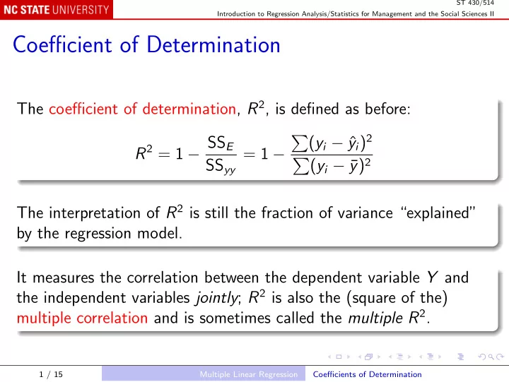
The coefficient of determination, R2, is defined as before: R2 = 1 − SSE SSyy = 1 − (yi − ˆ yi)2 (yi − ¯ y)2 The interpretation of R2 is still the fraction of variance “explained” by the regression model. It measures the correlation between the dependent variable Y and the independent variables jointly; R2 is also the (square of the) multiple correlation and is sometimes called the multiple R2.

1 / 15 Multiple Linear Regression Coefficients of Determination

ST 430/514 Introduction to Regression Analysis/Statistics for Management and the Social Sciences II

Adjusted Coefficient of Determination Because the regression model is adapted to the sample data, it tends to explain more variance in the sample data than it will in new data. Rewrite: 1 − R2 = SSE SSyy =

1 n

(yi − ˆ yi)2

1 n

(yi − ¯ y)2 Numerator and denominator are biased estimators of variance.

2 / 15 Multiple Linear Regression Coefficients of Determination

ST 430/514 Introduction to Regression Analysis/Statistics for Management and the Social Sciences II

Replace 1

n with the multipliers that give unbiased variance estimators: 1 n−p

(yi − ˆ yi)2

1 n−1

(yi − ¯ y)2 , where as before p = k + 1, the number of estimated βs. This defines the adjusted coefficient of determination: R2

a = 1 − 1 n−p

(yi − ˆ yi)2

1 n−1

(yi − ¯ y)2 = 1 − n − 1 n − p × (yi − ˆ yi)2 (yi − ¯ y)2 . R2

a < R2, and for a poorly fitting model you may even find R2 a < 0!

3 / 15 Multiple Linear Regression Coefficients of Determination

ST 430/514 Introduction to Regression Analysis/Statistics for Management and the Social Sciences II

Looking Ahead... To assess how well a model will predict new data, you can use deleted residuals (see Section 8.6, The Jackknife): Delete one observation, say yi; Refit the model, and use it to predict the deleted observation as ˆ y(i); The deleted residual (or prediction residual) is di = yi − ˆ y(i). More R2 (see Section 5.11, External Model Validation): R2

jackknife = 1 −

yi − ˆ y(i) 2 (yi − ¯ y)2 , P2 = 1 − yi − ˆ y(i) 2 yi − ¯ y(i) 2.

4 / 15 Multiple Linear Regression Coefficients of Determination

ST 430/514 Introduction to Regression Analysis/Statistics for Management and the Social Sciences II

A useful R function:

PRESS <- function(l) { r <- residuals(l) sse <- sum(r^2) d <- r / (1 - hatvalues(l)) press <- sum(d^2) sst <- sse / (1 - summary(l)$r.squared) n <- length(r) ssti <- sst * (n / (n - 1))^2 c(stat = press, pred.rmse = sqrt(press / n), pred.r.square = 1 - press / sst, P.square = 1 - press / ssti) }

5 / 15 Multiple Linear Regression Coefficients of Determination

ST 430/514 Introduction to Regression Analysis/Statistics for Management and the Social Sciences II

Estimation and Prediction

The multiple regression model may be used to make statements about the response that would be observed under a new set of conditions xnew = (x1,new, x2,new, . . . , xk,new). As before, the statement may be about: E(Y |x = xnew), the expected value of Y under the new conditions; a single new observation of Y under the new conditions.

6 / 15 Multiple Linear Regression Estimation and Prediction

ST 430/514 Introduction to Regression Analysis/Statistics for Management and the Social Sciences II

The point estimate of E(Y |x = xnew) and the point prediction of Y when x = xnew are both ˆ y = ˆ β0 + ˆ β1x1,new + · · · + ˆ βkxk,new. The standard errors are different because, as always, Y = E(Y ) + ǫ.

7 / 15 Multiple Linear Regression Estimation and Prediction

ST 430/514 Introduction to Regression Analysis/Statistics for Management and the Social Sciences II

Example: prices of grandfather clocks Get the data and plot them:

clocks = read.table("Text/Exercises&Examples/GFCLOCKS.txt", header = pairs(clocks[, c("PRICE", "AGE", "NUMBIDS")])

Fit the first-order model and summarize it:

clocksLm = lm(PRICE ~ AGE + NUMBIDS, clocks) summary(clocksLm) PRESS(clocksLm)

Check the residuals:

plot(clocksLm)

8 / 15 Multiple Linear Regression Estimation and Prediction

ST 430/514 Introduction to Regression Analysis/Statistics for Management and the Social Sciences II

Predictions are for an auction of a 150-year old clock with 10 bidders. 95% confidence interval for E(Y |AGE = 150, NUMBIDS = 10):

predict(clocksLm, newdata = data.frame(AGE = 150, NUMBIDS = 10), interval = "confidence", level = .95)

95% prediction interval for Y when AGE = 150, NUMBIDS = 10:

predict(clocksLm, newdata = data.frame(AGE = 150, NUMBIDS = 10), interval = "prediction", level = .95)

9 / 15 Multiple Linear Regression Estimation and Prediction

ST 430/514 Introduction to Regression Analysis/Statistics for Management and the Social Sciences II

Interaction Models

One property of the first-order model E(Y ) = β0 + β1x1 + β2x2 + · · · + βkxk is that βi is the change in E(Y ) as xi increases by 1 with all the

• ther independent variables held fixed, and is the same regardless of

the values of those other variables. Not all real-world situations work like that. When the magnitude of the effect of one variable is affected by the level of another, we say that they interact.

10 / 15 Multiple Linear Regression Interaction Model

ST 430/514 Introduction to Regression Analysis/Statistics for Management and the Social Sciences II

A simple model for two factors that interact is E(Y ) = β0 + β1x1 + β2x2 + β3x1x2. Rewrite this in two ways: E(Y ) = β0 + (β1 + β3x2)x1 + β2x2 = β0 + β1x1 + (β2 + β3x1)x2. Holding x2 fixed, the slope of E(Y ) against x1 is β1 + β3x2. Holding x1 fixed, the slope of E(Y ) against x2 is β2 + β3x1.

11 / 15 Multiple Linear Regression Interaction Model

ST 430/514 Introduction to Regression Analysis/Statistics for Management and the Social Sciences II

We can fit this using k = 3: E(Y ) = β0 + β1x1 + β2x2 + β3x3 if we set x3 = x1x2. Example: grandfather clocks again.

clocksLm2 <- lm(PRICE ~ AGE * NUMBIDS, clocks) summary(clocksLm2)

Note: the formula PRICE ˜ AGE * NUMBIDS specifies the interaction model, which includes the separate effects of AGE and NUMBIDS, together with their product, which will be labeled AGE:NUMBIDS.

12 / 15 Multiple Linear Regression Interaction Model

ST 430/514 Introduction to Regression Analysis/Statistics for Management and the Social Sciences II

Output

Call: lm(formula = PRICE ~ AGE * NUMBIDS, data = clocks) Residuals: Min 1Q Median 3Q Max

• 154.995
• 70.431

2.069 47.880 202.259 Coefficients: Estimate Std. Error t value Pr(>|t|) (Intercept) 320.4580 295.1413 1.086 0.28684 AGE 0.8781 2.0322 0.432 0.66896 NUMBIDS

• 93.2648

29.8916

• 3.120

0.00416 ** AGE:NUMBIDS 1.2978 0.2123 6.112 1.35e-06 ***

• Signif. codes:

0 *** 0.001 ** 0.01 * 0.05 . 0.1 1 Residual standard error: 88.91 on 28 degrees of freedom Multiple R-squared: 0.9539, Adjusted R-squared: 0.9489 F-statistic: 193 on 3 and 28 DF, p-value: < 2.2e-16

13 / 15 Multiple Linear Regression Interaction Model

ST 430/514 Introduction to Regression Analysis/Statistics for Management and the Social Sciences II

Note that the t-value on the AGE:NUMBIDS line is highly significant. That is, we strongly reject the null hypothesis H0 : β3 = 0. Effectively, this test is a comparison of the interaction model with the original non-interactive (additive) model. The other two t-statistics are usually irrelevant: if AGE:NUMBIDS is important, then both AGE and NUMBIDS should be included in the model; do not test the corresponding null hypotheses.

14 / 15 Multiple Linear Regression Interaction Model

ST 430/514 Introduction to Regression Analysis/Statistics for Management and the Social Sciences II

We can write the fitted model as E(PRICE) = 320 + (0.88 + 1.3 × NUMBIDS) × AGE − 93 × NUMBIDS meaning that the effect of age increases with the number of bidders. Check the model:

plot(clocksLm2)

More satisfactory than the additive model.

15 / 15 Multiple Linear Regression Interaction Model