10d Machine Learning: Symbol-based 10.0 Introduction 10.5 - PowerPoint PPT Presentation

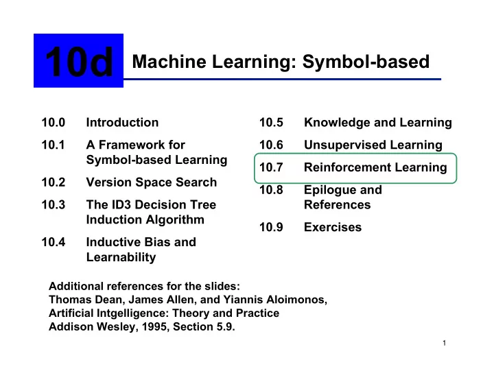
10d Machine Learning: Symbol-based 10.0 Introduction 10.5 Knowledge and Learning 10.1 A Framework for 10.6 Unsupervised Learning Symbol-based Learning 10.7 Reinforcement Learning 10.2 Version Space Search 10.8 Epilogue and 10.3 The ID3 Decision Tree References Induction Algorithm 10.9 Exercises 10.4 Inductive Bias and Learnability Additional references for the slides: Thomas Dean, James Allen, and Yiannis Aloimonos, Artificial Intgelligence: Theory and Practice Addison Wesley, 1995, Section 5.9. 1

Reinforcement Learning • A form of learning where the agent can explore and learn through interaction with the environment • The agent learns a policy which is a mapping from states to actions. The policy tells what the best move is in a particular state. • It is a general methodology: planning, decision making, search can all be viewed as some form of the reinforcement learning. 2

Tic-tac-toe: a different approach • Recall the minimax approach: The agent knows its current state. Generates a two layer search tree taking into account all the possible moves for itself and the opponent. Backs up values from the leaf nodes and takes the best move assuming that the opponent will also do so. • An alternative is to directly start playing with an opponent (does not have to be perfect, but could as well be). Assume no prior knowledge or lookahead. Assign “values” to states: 1 is win 0 is loss or draw 0.5 is anything else 3

Notice that 0.5 is arbitrary, it cannot differentiate between good moves and bad moves. So, the learner has no guidance initially. It engages in playing. When the game ends, if it is a win, the value 1 will be propagated backwards. If it is a draw or a loss, the value 0 is propagated backwards. Eventually, earlier states will be labeled to reflect their “true” value. After several plays, the learner will learn the best move given a state (a policy.)

Issues in generalizing this approach • How will the state values be initialized or propagated backwards? • What if there is no end to the game ( infinite horizon )? • This is an optimization problem which suggests that it is hard. How can an optimal policy be learned? 5

A simple robot domain The robot is in one of the states: 0, 1, 2, 3. Each one represents an office, the offices are connected in a @ @ ring. + 0 1 Three actions are available: - + moves to the “next” + - - + state - moves to the “previous” - state 3 2 @ remains at the same @ @ state + 6

The robot domain (cont’d) • The robot can observe the label of the state it is in and perform any action corresponding to an arc leading out of its current state. • We assume that there is a clock governing the passage of time, and that at each tick of the clock the robot has to perform an action. • The environment is deterministic , there is a unique state resulting from any initial state and action. • Each state has a reward : 10 for state 3, 0 for the others. 7

The reinforcement learning problem • Given information about the environment • States • Actions • State-transition function (or diagram) • Output a policy p: states → actions, i.e., find the best action to execute at each state • Assumes that the state is completely observable (the agent always knows which state it is in) 8

Compare three policies a. Every state is mapped to @ The value of this policy is 0, because the robot will never get to office 3. b. Every state is mapped to + policy 0 The value of this policy is ∞ , because the robot will end up in office 3 infinitely often. c. Every state is except 3 is mapped to +, 3 is mapped to @ policy 1 The value of this policy is also ∞ , because the robot will end up (stay) in office 3 infinitely often. 9

Compare three policies So, it is easy to rule case a out, but how can we show that policy 1 is better than policy 0? One way would be to compute the average reward per tick: POLICY 0 POLICY 1 The average reward per The average reward per tick for state 0 is 10/4. tick for state 0 is 10. Another way would be to assign higher values for immediate rewards and apply a discount to future rewards. 10

Discounted cumulative reward Assume that the robot associates a higher value with more immediate rewards and therefore discounts future rewards. The discount rate ( γ ) is a number between 0 and 1 used to discount future rewards. The discounted cumulative reward for a particular state with respect to a given policy is the sum for n from 0 to infinity of γ n times the reward associated with the state reached after the n-th tick of the clock. POLICY 0 POLICY 1 The discounted cumulative The discounted cumulative reward for state 0 is reward for state 0 is 1.33. 2.5. 11

Discounted cumulative reward (cont’d) Take γ = 0.5 For state 0 with respect to policy 0: 0.5 0 x 0 + 0.5 1 x 0 + 0.5 2 x 0 + 0.5 3 x 10 + 0.5 4 x 0 + 0.5 5 x 0 + 0.5 6 x 0 + 0.5 7 x 10 + … = 1.25 + 0.078 + … = 1.33 in the limit For state 0 with respect to policy 1: 0.5 0 x 0 + 0.5 1 x 0 + 0.5 2 x 0 + 0.5 3 x 10 + 0.5 4 x 10 + 0.5 5 x 10 + 0.5 6 x 10 + 0.5 7 x 10 + … = 2.5 in the limit 12

Discounted cumulative reward (cont’d) Let j be a state, R(j) be the reward for ending up in state j, π be a fixed policy, π (j) be the action dictated by π in state j, f(j,a) be the next state given the robot starts in state j and performs action a , V π i (j) be the estimated value of state j with respect to the policy π after the i-th iteration of the algorithm Using a dynamic programming algorithm, one can obtain a good estimate of V π , the value function for policy π as i → ∞ → ∞ . 13

A dynamic programming algorithm to compute values for states for a policy π 1. For each j, set V π 0 (j) to 0. 2. Set i to 0. 3. For each j, set V π i+1 (j) to R(j) + γ V π i ( f(j, π ) ) ) . 4. Set i to i + 1. 5. If i is equal to the maximum number of iterations, then return V π i otherwise, return to step 3. 14

Values of states for policy 0 • initialize • V(0) = 0 • V(1) = 0 • V(2) = 0 • V(3) = 0 • iteration 0 • For office 0: R(0) + γ V(1) = 0 + 0.5 x 0 = 0 • For office 1: R(1) + γ V(2) = 0 + 0.5 x 0 = 0 • For office 2: R(2) + γ V(3) = 0 + 0.5 x 0 = 0 • For office 3: R(3) + γ V(1) = 10 + 0.5 x 0 = 10 • (iteration 0 essentially initializes values of states to their immediate rewards) 15

Values of states for policy 0 (cont’d) • iteration 0 V(0) = V(1) = V(2) = 0 V(3)=10 • iteration 1 • For office 0: R(0) + γ V(1) = 0 + 0.5 x 0 = 0 • For office 1: R(1) + γ V(2) = 0 + 0.5 x 0 = 0 • For office 2: R(2) + γ V(3) = 0 + 0.5 x 10 = 5 • For office 3: R(3) + γ V(0) = 10 + 0.5 x 0 = 10 • iteration 2 • For office 0: R(0) + γ V(1) = 0 + 0.5 x 0 = 0 • For office 1: R(1) + γ V(2) = 0 + 0.5 x 5 = 2.5 • For office 2: R(2) + γ V(3) = 0 + 0.5 x 10 = 5 • For office 3: R(3) + γ V(0) = 10 + 0.5 x 0 = 10 16

Values of states for policy 0 (cont’d) • iteration 2 V(0) = 0 V(1) = 2.5 V(2) = 5 V(3) = 10 • iteration 3 • For office 0: R(0) + γ V(1) = 0 + 0.5 x 2.5 = 1.25 • For office 1: R(1) + γ V(2) = 0 + 0.5 x 5 = 2.5 • For office 2: R(2) + γ V(3) = 0 + 0.5 x 10 = 5 • For office 3: R(3) + γ V(0) = 10 + 0.5 x 0 = 10 • iteration 4 • For office 0: R(0) + γ V(1) = 0 + 0.5 x 2.5 = 1.25 • For office 1: R(1) + γ V(2) = 0 + 0.5 x 5 = 2.5 • For office 2: R(2) + γ V(3) = 0 + 0.5 x 10 = 5 • For office 3: R(3) + γ V(1) = 10 + 0.5 x 1.25 = 10.625 17

Values of states for policy 1 • initialize • V(0) = 0 • V(1) = 0 • V(2) = 0 • V(3) = 0 • iteration 0 • For office 0: R(0) + γ V(1) = 0 + 0.5 x 0 = 0 • For office 1: R(1) + γ V(2) = 0 + 0.5 x 0 = 0 • For office 2: R(2) + γ V(3) = 0 + 0.5 x 0 = 0 • For office 3: R(3) + γ V(3) = 10 + 0.5 x 0 = 10 18

Values of states for policy 1 (cont’d) • iteration 0 V(0) = V(1) = V(2) = 0 V(3)=15 • iteration 1 • For office 0: R(0) + γ V(1) = 0 + 0.5 x 0 = 0 • For office 1: R(1) + γ V(2) = 0 + 0.5 x 0 = 0 • For office 2: R(2) + γ V(3) = 0 + 0.5 x 10 = 5 • For office 3: R(3) + γ V(3) = 10 + 0.5 x 10 = 15 • iteration 2 • For office 0: R(0) + γ V(1) = 0 + 0.5 x 0 = 0 • For office 1: R(1) + γ V(2) = 0 + 0.5 x 5 = 2.5 • For office 2: R(2) + γ V(3) = 0 + 0.5 x 15 = 7.5 • For office 3: R(3) + γ V(3) = 10 + 0.5 x 15 = 17.5 19

Values of states for policy 1 (cont’d) • iteration 2 V(0) = 0 V(1) = 2.5 V(2) = 7.5 V(3) = 17.5 • iteration 3 • For office 0: R(0) + γ V(1) = 0 + 0.5 x 2.5 = 1.25 • For office 1: R(1) + γ V(2) = 0 + 0.5 x 7.5 = 3.75 • For office 2: R(2) + γ V(3) = 0 + 0.5 x 17.5 = 8.75 • For office 3: R(3) + γ V(3) = 10 + 0.5 x 17.5 = 18.75 • iteration 4 • For office 0: R(0) + γ V(1) = 0 + 0.5 x 3.75 = 1.875 • For office 1: R(1) + γ V(2) = 0 + 0.5 x 8.75 = 4.375 • For office 2: R(2) + γ V(3) = 0 + 0.5 x 18.75 = 9.375 • For office 3: R(3) + γ V(3) = 10 + 0.5 x 18.75 = 19.375 20