Buoyancy and vertical motion in a fluid In the atmosphere, local - - PowerPoint PPT Presentation

Buoyancy and vertical motion in a fluid

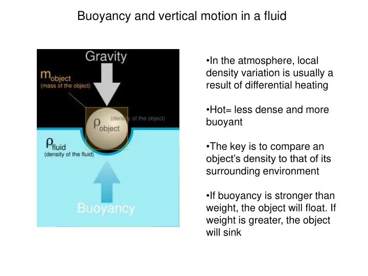
• In the atmosphere, local

density variation is usually a result of differential heating

• Hot= less dense and more

buoyant

• The key is to compare an
• bject’s density to that of its

surrounding environment

• If buoyancy is stronger than

weight, the object will float. If weight is greater, the object will sink

What is a parcel How is buoyancy defined?

• A “parcel” of air is like a bubble of air that rises upward from

near the surface through the atmosphere. Much of atmospheric convection can be understood by analyzing the behavior of a rising parcel

• Buoyancy is the vertical force caused by density difference

between “parcel” and surrounding environment that causes it to rise

• F=m a (Newton’s 2nd law)

e e p t environmen parcel t environmen buoyancy

T T T a

3 different lapse rates to keep track of:

Environmental Lapse Rate: 6.5 C/km

• Caused by radiation balances between surface and
• troposphere and atmospheric conditions
• Dramatic variance from day to day results in much of our weather
• “The reason we launch weather balloons”

Dry Adiabatic Lapse Rate: 9.8 C/km

• Combination of 1st law of Thermodynamics, ideal gas law and pressure change with height
• As air expands, molecules are spread apart and slow down (conservation of energy)
• “Rising Air Cools”

Moist Adiabatic Lapse Rate: ~6 C/km

• Condensation of cloud drops releases latent heat, reducing cooling
• Value changes slightly w/height and T because of variable condensation rate
• Positive feedback for instability
• “Rising clouds cool, but not as much”

3 different types of stability to remember

Absolutely Stable: Γenv<6 °C/km

• When lapse rate of the environment is low, causing air to cool with height more slowly than

any kind of parcel

• As a parcel rises it will become colder faster than the environment and quickly become

more dense than surroundings, causing it to sink.

• Cumulus clouds can’t form spontaneously when absolutely stable conditions exist

Absolutely Unstable: Γenv>9.8 °C/km

• When lapse rate of the environment is high, rising air cools, but not as quickly as the

surroundings.

• The rising parcel experiences a greater and greater density deficit, causing rapid upward

acceleration

• If absolute instability occurs over a large depth of the atmosphere, look out!

Conditional Stability: 6 °C/km < Γenv< 9.8 °C/km

• When the atmosphere has an intermediate lapse rate (typical) it will allow cool slower than

condensing air but faster than dry air.

• Once a cloud has formed, it can continue to rise and develop on its own because of the

density deficit.

• Dry air won’t rise on its own, but if it can be forced upward some other way to generate

clouds, then convection can take off. This occurs frequently.

Environment and Parcel Lines:

• When parcel line is to the right (warmer), buoyancy is positive
• Slope of line shows lapse rates
• Area between lines shows magnitude of accumulated buoyancy
• Cloud forms at “Lifting Condensation Level” – Cloud base, determined only be

dewpoint depression; rule of thumb: LCL (1000’s of ft) = (T-Td)/4.4

Environment and Parcel Lines:

• When parcel line is to the left (colder), buoyancy is negative
• Air won’t rise unless it is forced to rise in another way (i.e convergence)

Environment and Parcel Lines:

• Conditional Instability can result in convection if low-level forcing can initial

condensation

• “Level of Free Convection”

Stable or Unstable?

Generally, what can a skew-T diagram tell us?

• Upper-level temperature, moisture, pressure and wind
• Stability of the atmosphere, and therefore probability of Tstorms
• Lower atmosphere temps, and therefore frozen precip. Type
• Wind speed with height, and therefore tornadic possibility or aviation turbulence
• Likelihood and altitude of cloudiness in the absence of convection
• Where in the atmosphere clouds are likely to transition to mixed and solid phase

Specifically, what markers are we looking for?

• T and Td at any level
• Wind speed and dir at any level
• Lapse rates at various levels
• LCL: Lifting Condensation Level
• CCL: Convective Condensation Level
• LFC: Level of Free Convection
• CAPE: Convective Available Potential Energy
• CIN: Convective Inhibition
• EL: Equilibrium Level
• MPL: Max. Parcel Height
• FZL: Freezing Level
• WBZ: Wet Bulb Zero Level
• PW: Precipitable Water
• CONVT: Convective Temperature

Lifting Condensation Level?

• Follow the surface mixing ratio upwards until it

intersects with the dry adiabatic lapse rate of the lifted (and cooling) surface parcel

• This intersection indicates that the parcel has

been lifted to its saturation mixing ratio and condensation will occur

• This estimates the cloud base from surface

convection or surface-lifting

• Try it on your skew-T – what do you get

Convective Condensation Level?

• Follow the surface mixing ratio upwards until it

intersects with the temperature sounding itself.

• This intersection indicates that the saturation is

reached in a parcel rising from the surface on its

• wn later in the day – this parcel would have to be

warmer than the surface at the time of the sounding, which results in a higher cloud base

• This estimates the cloud base from afternoon

surface convection better than the LCL

• Try it on your skew-T – what do you get

Level of Free Convection:

• From the LCL, the parcel will now cool along a

moist adiabat

• Follow the moist adiabat until the parcel’s

Temperature crosses that of the environment

• At this point the parcel is buoyant and an updraft

will result

• This won’t occur on soundings that are stable
• Find the LFC on your skew-T

Convective Available Potential Energy?

• Find the area between the parcel and environment above the LFC until

the temperatures intersect again.

• Because temperature is proportional to density, this equation integrates

buoyancy force X distance which is an energy

• This “potential energy” gets converted to kinetic energy in the updraft
• Greater CAPE = stronger updrafts and storms
• Difference between “tall and skinny and tall and fat CAPE”
• This is the best measurement of instability for storm formation
• Shade the CAPE on your skew T

Convective Inhibition?

• CIN is pretty much the opposite of CAPE– this is negative buoyancy area

that acts to prevent convection

• This is the area between the environmental and parcel temperature

that is below the LFC, where the parcel is colder

• Greater values of CIN require extraordinary lifting to get through
• Some moderate CIN can actually promote explosive storm development

if there is big CAPE above the CIN

• Like busting down a door

Equilibrium Level?

• EL is the second crossing of parcel and

environmental Temperature

• The parcel is now neutrally buoyant – it is still

moving up, but no longer accelerating

• This is where the cloud top starts to slow down its

upward movement

• Try it on your skew-T – what do you get

• Max. Parcel Level?
• MPL is the highest level a convective cloud might reach if

it taps into all of the available instability

• This occurs where the negative bouyancy above the EL

balances out the CAPE below it…the parcel is decelerated to zero.

• This is the maximum convective cloud top height – an

important parameter for aviation. The higher the cloud top, the greater the updraft must have been.

• Try it on your skew-T – what do you get

Freezing Level

• FZL The height/pressure where the sounding indicates

that the environment drops below 0 C

• Above this temperature, mixed phase clouds are possible
• Convective clouds likely need to reach at least -20 C to

beginning generating charge separation

• Cirrus clouds are not likely until you reach -30 C
• The location of this level is important in marginal frozen
• precip. forecasts
• Try it on your skew-T – what do you get

Wet bulb zero level

• WBZ is the level where the wet-bulb temperature of the

environment is 0 C

• This is an important value for determining frozen precip.

type

• Falling precipitation causes evaporative cooling of the

surrounding air – the wet bulb temperature shows how much cooling potential exists. This effect allows “dynamic cooling” during heavy precipitation and may permit snow even if the sounding shows marginally above freezing temps.

• Try it on your skew-T – what do you get

Precipitable Water?

• PW is an integration of the total amount of water

vapor in the sounding if it where all condensed

• Greater precipitable water is likely to promote

heavy rain events

• Not easy to estimate on your own – just read it
• ff the plot analysis

Convective Temperature

• This is the temperature the surface would have

to reach so that the parcel could rise on its own – essentially bringing the LFC to the surface

• If this value is indicated on a morning sounding

and the expected afternoon temperature is greater than this value, convection is highly likely.

Where can you get skew-T’s and cloud height information?

• Storm Prediction Center—Forecast tools
• NOAA UCAR – upper air data