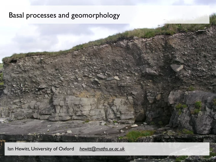
Basal processes and geomorphology Ian Hewitt, University of Oxford - PowerPoint PPT Presentation

Basal processes and geomorphology Ian Hewitt, University of Oxford hewitt@maths.ox.ac.uk 1

Sediments and sliding - Till rheology - Deformation Drainage in sediments - Darcy flow - Canals Geomorphology - Meltwater deposits - Deformational deposits 2

Sediments and sliding 3

Basal sediments Many glaciers and ice sheets have a layer of sediments (till) at the bed eg. Siple coast ice streams, Iceland, Svalbard Sediments result from glacial erosion (eg. abrasion, plucking) Midtre Lovenbreen, Glaciers Online Samples suggest a poorly sorted spectrum of grain sizes (fractal dimension ~2.9) Till is often water saturated Deformation Sometimes the water may be frozen (it may be hard to say where ‘ice-till’ interface is!) Hooke & Iverson 1995 4

Sliding over sediments τ b β u b ‘Sliding’ could involve: τ b - Shear deformation of sediment layer h T U b τ b β u b τ b U b - Shear of a finite horizon of the sediment h T τ b β u b - Slip at the ice-till interface Macroscopic resistance may come from flow around sediment landforms τ b β u b τ b β u b - Slip on slip-planes within the sediment layer 5

Till rheology Hooke & Iverson 1998, Kamb 1991, Iverson 2011 Till rheology has been a subject of some controversy Laboratory experiments on samples show that till has a yield stress τ f = c 0 + µ σ e ⇥ Yield stress depends on effective stress σ e = P � p w p w ⇥ N Effective pressure at ice-till interface (effective stress increases with depth into the till - it is weakest at the top). � Coefficient of friction µ = tan ψ ⇥ 0 . 4 ⇥ Cohesion c 0 ⇥ 3 kPa Experiments suggest stress is largely independent of strain rate (i.e. perfectly plastic). Iverson et al 1998, Clarke 2005 6

Till rheology Boulton & Hindmarsh 1987, Kamb 1991 It is desirable to have some way of describing plastic flow when the yield stress is exceeded. ⇥ σ e Stress τ Boulton & Hindmarsh popularized a power law rheology � a = 1 . 33 ε = A ( τ � τ f ) a σ − b ˙ τ f = µ σ e e τ f b = 1 . 8 It is questionable whether there is enough data to confirm such a relationship. Strain rate ˙ ε ⇥ σ e Stress τ Kamb suggested an exponential relationship (following critical-state soil mechanics theory) τ f τ f = µ σ e ε = A exp ( ατ / τ f ) ˙ ⇥ ie. almost perfectly Experiments suggest Strain rate ˙ a ⇥ α ⇥ 75 ε plastic. 7

Sliding over till Basal shear σ e τ b β u b stress τ b Viscous rheology � ε = A ( τ � τ f ) a σ − b τ f ˙ τ ⇥ τ f = µ σ e e h T Pore water pressure roughly hydrostatic Sliding speed U b Effective stress increases with depth through till σ e = N + ∆ ρ sw g ( Z b − z ) � Deformation only if Deforming horizon h T = [ τ b � µN ] + /µ ∆ ρ sw g σ e ≤ τ b /µ Sliding law τ b = µN + CU 1 /a N b/a b τ b β u b A similar law applies to describe ice flow τ b = µN + RU 1 /n over sediments with topography b Numerical models often use a `pseudo-plastic’ law τ b = CU q q ⌧ 1 b 8

Meltwater drainage 9

Drainage through till Estimates of till conductivity vary considerably, but it is generally thought to be low. Although water seeps vertically into the till, horizontal transport through the till is insufficient to evacuate the water produced from melting. eg. in Antarctica m s − 1 m q ⌅ 10 − 7 · 10 Pa q = Kh T m ⌅ 10 − 10 m 2 s − 1 10 3 · 10 · 10 ρ w g ⇧ φ kg m − 3 m s − 2 − − · ⇤ m d x ⌅ 5 · 10 3 mm y − 1 km ⌅ 1 . 6 ⇥ 10 − 4 m 2 s − 1 Water flows in a patchy film at the ice-till interface, or in some form of channels or canals . Canals Walder & Fowler 1994 Patchy sheet Alley 1989, Creyts & Schoof 2009 10

Canals Walder & Fowler 1994, Ng 2000 Gravitational potential gradient � ∂ x ∂ x Creep Ψ = ρ i g tan α + ( ρ w � ρ i ) g tan θ Melting Erosion Creep Walder & Fowler suggested two possibilities for steady states: ⇧ G Channels - mostly melted into ice N > ˜ N / Ψ 7 / 15 Q 1 / 15 N ˜ N ⇤ 0 . 8 MPa / N / Ψ − 1 / 3 Q − 1 / 3 Canals - mostly eroded into sediment N < ˜ N Effective pressure in canals DECREASES with increasing discharge Q Q The crucial difference is that sediment erosion tends to produce a wide cross-section . Canals are favoured when the potential gradient is small (e.g. interior of ice sheets). 11

Interaction of sliding and drainage ∂ N A consequence of is the potential for a positive feedback ∂ Q < 0 Positive feedback Initiation of sliding U b Increased melting m ∝ τ b U b /L τ b = CU p b N q ∝ Increased discharge � Q Lower effective pressure N Model U b Q = G + τ b U b − kU 1 / 2 Fast moving, b A ρ w L lots of water N = c/Q 1 / 3 ⌅ Slow moving, τ b = CU p b N q not much water The relationship between ice thickness and speed τ b ≈ − ρ i gh ∂ s can become multivalued ∂ x 12

Surges and ice streaming Temporal variability − Q i accumulation ∝ − d h d t ∝ A − Q i Heinrich events, surges ice flux MacAyeal 1992 ∝ h Spatial variability Ice streams \ 13

Meltwater deposits 14

Meltwater deposits Creep Deposition of sediments in Röthlisberger channels can build eskers Melting - Most likely under falling water speed, near margin - Sediment is flushed from the surrounding bed - Esker size depends on margin retreat rate Deposition Creep Erosion of sediments from canals can create tunnel valleys Melting Erosion Creep Creep Erosion 15

Eskers Canadian eskers form predominantly on crystalline bedrock. Probably reflects channelised drainage Clark & Walder 1994 Storrar et al 2014 Bridgenorth Esker 16

Eskers Melting Ice Esker Sediments Subglacial channel Retreat Model An extended version of the Röthlisberger channel model that incorporates sediment transport. Hewitt & Creyts 2019 Geophys. Res. Lett. 17

Eskers Sediment deposition acts to clog the channel: ∂ S ∂ t = Q Ψ ASN n � D ρ i L � ˜ m V S S Q A A x Q s ∂ A ∂ t = D ! V m Hewitt & Creyts 2019 Geophys. Res. Lett. Boundary-layer analysis leads (….) to an A = C Q − 4 / 5 Q 29 / 15 V − 1 approximation of the cross-sectional area: m s m m Retreat rate Meltwater flux Sediment flux Esker size increases roughly quadratically with sediment flux , decreases roughly linearly with meltwater flux , and decreases linearly with ice-sheet retreat rate . 18

Deformational deposits 19

Drumlins Subglacial waveforms formed by deformation/erosion by ice flow 20

Drumlins King et al 2007 Inferred drumlin beneath Rutford ice stream from seismic survey Smith et al 2007 21

Mega-scale glacial lineations Radar profile of bed beneath Rutford ice stream (West Antarctica) compared with de-glaciated bed of former ice stream. 5,000 m Bed elevation (m) E W ¬1,700 Dilatant till/ ¬1,900 Rutford Ice Stream Dubawnt Lake, Canada deforming bed Stiff till/basal sliding ¬2,100 n o i t c e r i d n o w i t o c l 5,000 m e f r e i 500 m d c I w o l f e c I Ice flow 5 km 5 km 5 , 0 0 0 m direction King et al 2009 22

� � � � � � � � � � � � � � � Instability theory Hindmarsh 1998, Schoof 2007, Fowler 2000, 2001, 2002, 2009, 2010, 2010, Fowler & Chapwanya 2014 � � � U � q s N ∂ s ∂ t + ∂ q Conservation of sediment Sediment flux q = q ( τ , N ) ∂ x = 0 Sliding law � τ = τ ( U, N ) � � � � U � � ∂τ > ∂τ Instability if � � � � ∂ N ∂ N � � U q 23 � � � � � � � �

Instability theory Fowler & Chapwanya 2014 Modified theory may explain evolution of ribbed moraine, drumlins, and mega-scale lineations σ ( h 3 ) x = V .[ h 3 V ψ ],      Ψ = s − N + Φ ,       � f ( ¯ � A = 1 u , N )   − N ,    2 µ  +      ε rh t = 1 − Π hN , (2.59)  b = s − δ h ,       u i ] + σγ [ B ( τ e ) h ] x = β V .[ A 3 V N ] + γ V .[ B ( τ e ) { h V Ψ + θ V b } ],  b t + V .[ A ¯       τ e = σ h i − { h V Ψ + θ V b }        α s t + ¯ us x = w ( Φ , N ). - Ice flow over sediments causes transverse dune-like instability. - Water flow carrying sediments causes longitudinal rill-like instability. ( a ) r i b s , P = 0.7 ( b ) ( c ) MSGL, P = 10 Growth rates dr u ml i n s , P = 2 10 8 20 10 2.5 5 7 8 2.0 6 8 4 15 5 1.5 6 3 6 4 1.0 k 2 k 2 k 2 10 3 2 4 0.5 4 2 1 0 5 1 2 2 –0.5 0 0 –1 –1.0 –1 –1 0 2 4 6 8 10 0 5 10 15 20 0 2 4 6 8 10 k 1 k 1 k 1 24 MSGL, P = 10

Instability theory Barchyn et al 2016 Barchyn et al 2016 25

Summary Friction laws for soft beds are similar to hard-bed sliding laws (even though the local slip / deformation mechanism may be different). Drainage over till may occur through films, cavities and canals. Eskers form through deposition in Röthlisberger channels. Tunnel valleys form through excess erosion in canals. Ice flow over deforming till can be unstable and produce ribbed moraine, drumlins, and mega-scale glacial lineations. An important (unsolved) question is how the development of these bed- forms controls/affects ice dynamics. 26