
SLIDE 1
Automation Lab IIT Bombay
System Identification 99 4/10/2012 System Identification 99
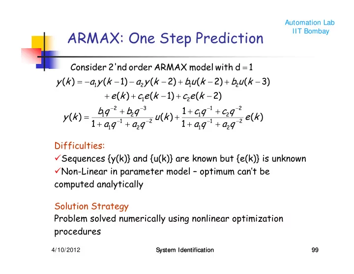
ARMAX: One Step Prediction
) ( 1 1 ) ( 1 ) ( ) 2 ( ) 1 ( ) ( ) 3 ( ) 2 ( ) 2 ( ) 1 ( ) ( 1 d with model ARMAX
- rder
nd 2' Consider
2 2 1 1 2 2 1 1 2 2 1 1 3 2 2 1 2 1 2 1 2 1
k e q a q a q c q c k u q a q a q b q b k y k e c k e c k e k u b k u b k y a k y a k y
− − − − − − − −