A comparison with LP (I) Example (Prolog): q(X, Y, Z) :- Z = f(X, - PowerPoint PPT Presentation

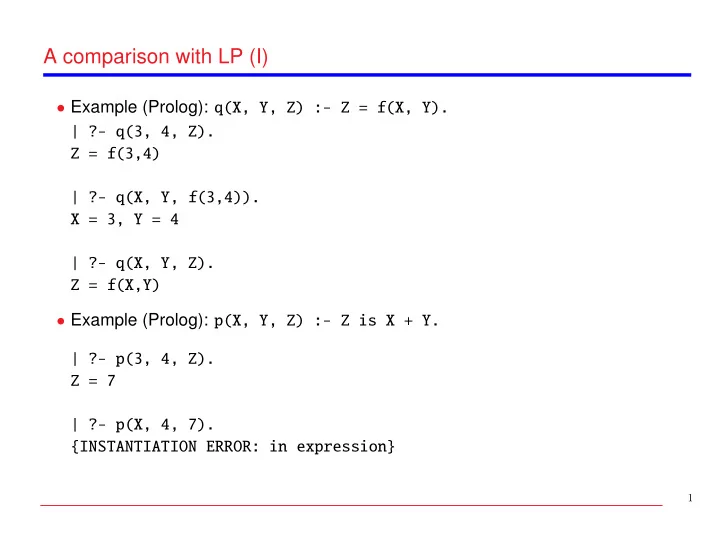
A comparison with LP (I) • Example (Prolog): q(X, Y, Z) :- Z = f(X, Y). | ?- q(3, 4, Z). Z = f(3,4) | ?- q(X, Y, f(3,4)). X = 3, Y = 4 | ?- q(X, Y, Z). Z = f(X,Y) • Example (Prolog): p(X, Y, Z) :- Z is X + Y. | ?- p(3, 4, Z). Z = 7 | ?- p(X, 4, 7). {INSTANTIATION ERROR: in expression} 1

A Comparison with LP (II) • Example (CLP( ℜ )): p(X, Y, Z) :- Z = X + Y. 2 ?- p(3, 4, Z). Z = 7 *** Yes 3 ?- p(X, 4, 7). X = 3 *** Yes 4 ?- p(X, Y, 7). X = 7 - Y *** Yes 2

A Comparison with LP (III) • Features in CLP: ⋄ Domain of computation (reals, integers, booleans, etc). Have to meet some conditions. ⋄ Type of constraints allowed for each domain: e.g. arithmetic constraints ( + , ∗ , = , ≤ , ≥ , <, > ) ⋄ Constraint solving algorithms: simplex, gauss, etc. • LP can be viewed as a constraint logic language over Herbrand terms with a single constraint predicate symbol: “=” 3

A Comparison with LP (IV) • Advantages: ⋄ Helps making programs expressive and flexible. ⋄ May save much coding. ⋄ In some cases, more efficient than traditional LP programs due to solvers typically being very efficiently implemented. ⋄ Also, efficiency due to search space reduction: * LP: generate-and-test. * CLP: constrain-and-generate. • Disadvantages: ⋄ Complexity of solver algorithms (simplex, gauss, etc) for system developer (and can affect performance). 4

Example of Search Space Reduction • Prolog (generate–and–test): solution(X, Y, Z) :- p(X), p(Y), p(Z), test(X, Y, Z). p(14). p(15). p(16). p(7). p(3). p(11). test(X, Y, Z) :- Y is X + 1, Z is Y + 1. • Query: | ?- solution(X, Y, Z). X = 14 Y = 15 Z = 16 ? ; no • 458 steps (all solutions: 465 steps). 5

Example of Search Space Reduction • CLP( ℜ ) (using generate–and–test): solution(X, Y, Z) :- p(X), p(Y), p(Z), test(X, Y, Z). p(14). p(15). p(16). p(7). p(3). p(11). test(X, Y, Z) :- Y = X + 1, Z = Y + 1. • Query: ?- solution(X, Y, Z). Z = 16 Y = 15 X = 14 *** Retry? y *** No • 458 steps (all solutions: 465 steps). 6

Generate–and–test Search Tree g X=14 X=15 X=16 X=7 X=3 X=11 A5 A4 A3 A2 A1 A Y=14 Y=15 Y=16 Y=7 Y=3 Y=11 B5 B4 B3 B2 B1 B Z=14 Z=15 Z=16 Z=7 Z=3 Z=11 7

Example of Search Space Reduction • Move test(X, Y, Z) at the beginning (constrain–and–generate): solution(X, Y, Z) :- test(X, Y, Z), p(X), p(Y), p(Z). p(14). p(15). p(16). p(7). p(3). p(11). • Prolog: test(X, Y, Z) :- Y is X + 1, Z is Y + 1. | ?- solution(X, Y, Z). {INSTANTIATION ERROR: in expression} • CLP( ℜ ): test(X, Y, Z) :- Y = X + 1, Z = Y + 1. ?- solution(X, Y, Z). Z = 16 Y = 15 X = 14 *** Retry? y *** No • 11 steps (all solutions: 11 steps). 8

Constrain–and–generate Search Tree g X=14 X=15 X=16 X=7 X=3 X=11 Y=15 Y=16 Z=16 9

Fibonaci Revisited (Prolog) • Fibonaci numbers: F 0 = 0 F 1 = 1 F n +2 = F n +1 + F n • (The good old) Prolog version: fib(0, 0). fib(1, 1). fib(N, F) :- N > 1, N1 is N - 1, N2 is N - 2, fib(N1, F1), fib(N2, F2), F is F1 + F2. • Can only be used with the first argument instantiated to a number 10

Fibonaci Revisited (CLP( ℜ )) • CLP( ℜ ) version: syntactically similar to the previous one fib(0, 0). fib(1, 1). fib(N, F1 + F2) :- N > 1, F1 >= 0, F2 >= 0, fib(N - 1, F1), fib(N - 2, F2). • Note all constraints included in program ( F1 >= 0, F2 >= 0 ) – good practice! • Only real numbers and equations used (no data structures, no other constraint system): “pure CLP( ℜ )” • Semantics greatly enhanced! E.g. ?- fib(N, F). F = 0, N = 0 ; F = 1, N = 1 ; F = 1, N = 2 ; F = 2, N = 3 ; F = 3, N = 4 ; 11

Analog RLC circuits (CLP( ℜ )) • Analysis and synthesis of analog circuits • RLC network in steady state • Each circuit is composed either of: ⋄ A simple component, or ⋄ A connection of simpler circuits • For simplicity, we will suppose subnetworks connected only in parallel and series − → Ohm’s laws will suffice (other networks need global, i.e., Kirchoff’s laws) • We want to relate the current ( I ), voltage ( V ) and frequency ( W ) in steady state • Entry point: circuit(C, V, I, W) states that: across the network C , the voltage is V , the current is I and the frequency is W • V and I must be modeled as complex numbers (the imaginary part takes into account the angular frequency) • Note that Herbrand terms are used to provide data structures 12

Analog RLC circuits (CLP( ℜ )) • Complex number X + Y i modeled as c(X, Y) • Basic operations: c_add(c(Re1,Im1), c(Re2,Im2), c(Re1+Re2,Im1+Im2)). c_mult(c(Re1, Im1), c(Re2, Im2), c(Re3, Im3)) :- Re3 = Re1 * Re2 - Im1 * Im2, Im3 = Re1 * Im2 + Re2 * Im1. (equality is c equal(c(R, I), c(R, I)) , can be left to [extended] unification) 13

Analog RLC circuits (CLP( ℜ )) • Circuits in series: circuit(series(N1, N2), V, I, W) :- c_add(V1, V2, V), circuit(N1, V1, I, W), circuit(N2, V2, I, W). • Circuits in parallel: circuit(parallel(N1, N2), V, I, W) :- c_add(I1, I2, I), circuit(N1, V, I1, W), circuit(N2, V, I2, W). 14

Analog RLC circuits (CLP( ℜ )) Each basic component can be modeled as a separate unit: • Resistor: V = I ∗ ( R + 0 i ) circuit(resistor(R), V, I, _W) :- c_mult(I, c(R, 0), V). • Inductor: V = I ∗ (0 + WLi ) circuit(inductor(L), V, I, W) :- c_mult(I, c(0, W * L), V). 1 • Capacitor: V = I ∗ (0 − WC i ) circuit(capacitor(C), V, I, W) :- c_mult(I, c(0, -1 / (W * C)), V). 15

Analog RLC circuits (CLP( ℜ )) • Example: R = ? C = ? V = 4.5 ω = 2400 I = 0.65 L = 0.073 ?- circuit(parallel(inductor(0.073), series(capacitor(C), resistor(R))), c(4.5, 0), c(0.65, 0), 2400). R = 6.91229, C = 0.00152546 ?- circuit(C, c(4.5, 0), c(0.65, 0), 2400). 16

The N Queens Problem • Problem: place N chess queens in a N × N board such that they do not attack each other • Data structure: a list holding the column position for each row • The final solution is a permutation of the list [1, 2, ..., N] • E.g.: the solution is represented as [2, 4, 1, 3] • General idea: ⋄ Start with partial solution ⋄ Nondeterministically select new queen ⋄ Check safety of new queen against those already placed ⋄ Add new queen to partial solution if compatible; start again with new partial solution 17

The N Queens Problem (Prolog) queens(N, Qs) :- queens_list(N, Ns), queens(Ns, [], Qs). queens([], Qs, Qs). queens(Unplaced, Placed, Qs) :- select(Unplaced, Q, NewUnplaced), no_attack(Placed, Q, 1), queens(NewUnplaced, [Q|Placed], Qs). no_attack([], _Queen, _Nb). no_attack([Y|Ys], Queen, Nb) :- Queen =\= Y + Nb, Queen =\= Y - Nb, Nb1 is Nb + 1, no_attack(Ys, Queen, Nb1). select([X|Ys], X, Ys). select([Y|Ys], X, [Y|Zs]) :- select(Ys, X, Zs). queens_list(0, []). queens_list(N, [N|Ns]) :- N > 0, N1 is N - 1, queens_list(N1, Ns). 18

The N Queens Problem (Prolog) 19

The N Queens Problem (CLP( ℜ )) queens(N, Qs) :- constrain_values(N, N, Qs), place_queens(N, Qs). constrain_values(0, _N, []). constrain_values(N, Range, [X|Xs]) :- N > 0, X > 0, X <= Range, constrain_values(N - 1, Range, Xs), no_attack(Xs, X, 1). no_attack([], _Queen, _Nb). no_attack([Y|Ys], Queen, Nb) :- abs(Queen - (Y + Nb)) > 0, % Queen =\= Y + Nb abs(Queen - (Y - Nb)) > 0, % Queen =\= Y - Nb no_attack(Ys, Queen, Nb + 1). place_queens(0, _). place_queens(N, Q) :- N > 0, member(N, Q), place_queens(N - 1, Q). member(X, [X|_]). member(X, [_|Xs]) :- member(X, Xs). 20

The N Queens Problem (CLP( ℜ )) • This last program can attack the problem in its most general instance: ?- queens(M,N). N = [], M = 0 ; M = [1], M = 1 ; N = [2, 4, 1, 3], M = 4 ; N = [3, 1, 4, 2], M = 4 ; N = [5, 2, 4, 1, 3], M = 5 ; N = [5, 3, 1, 4, 2], M = 5 ; N = [3, 5, 2, 4, 1], M = 5 ; N = [2, 5, 3, 1, 4], M = 5 ... • Remark: Herbrand terms used to build the data structures • But also used as constraints (e.g., length of already built list Xs in no attack(Xs, X, 1) ) • Note that in fact we are using both ℜ and FT 21

The N Queens Problem (CLP( ℜ )) 22

The N Queens Problem (CLP( ℜ )) • CLP( ℜ ) generates internally a set of equations for each board size • They are non–linear and are thus delayed until instantiation wakes them up ?- constrain_values(4, 4, Q). Q = [_t3, _t5, _t13, _t21] _t3 <= 4 0 < abs(-_t13 + _t3 - 2) _t5 <= 4 0 < abs(-_t13 + _t3 + 2) _t13 <= 4 0 < abs(-_t21 + _t3 - 3) _t21 <= 4 0 < abs(-_t21 + _t3 + 3) 0 < _t3 0 < abs(-_t13 + _t5 - 1) 0 < _t5 0 < abs(-_t13 + _t5 + 1) 0 < _t13 0 < abs(-_t21 + _t5 - 2) 0 < _t21 0 < abs(-_t21 + _t5 + 2) 0 < abs(-_t5 + _t3 - 1) 0 < abs(-_t21 + _t13 - 1) 0 < abs(-_t5 + _t3 + 1) 0 < abs(-_t21 + _t13 + 1) 23

The N Queens Problem (CLP( ℜ )) • Constraints are (incrementally) simplified as new queens are added ?- constrain_values(4, 4, Qs), Qs = [3,1|OQs]. OQs = [_t16, _t24] 0 < abs(-_t24) Qs = [3, 1, _t16, _t24] 0 < abs(-_t24 + 6) _t16 <= 4 0 < abs(-_t16) _t24 <= 4 0 < abs(-_t16 + 2) 0 < _t16 0 < abs(-_t24 - 1) 0 < _t24 0 < abs(-_t24 + 3) 0 < abs(-_t16 + 1) 0 < abs(-_t24 + _t16 - 1) 0 < abs(-_t16 + 5) 0 < abs(-_t24 + _t16 + 1) • Bad choices are rejected using constraint consistency: ?- constrain_values(4, 4, Qs), Qs = [3,2|OQs]. *** No 24