10 12 2019
play

10-12-2019 Motivation Dairy cow mastitis is a serious problem - PDF document

10-12-2019 Motivation Dairy cow mastitis is a serious problem Financial loss Animal welfare issue 
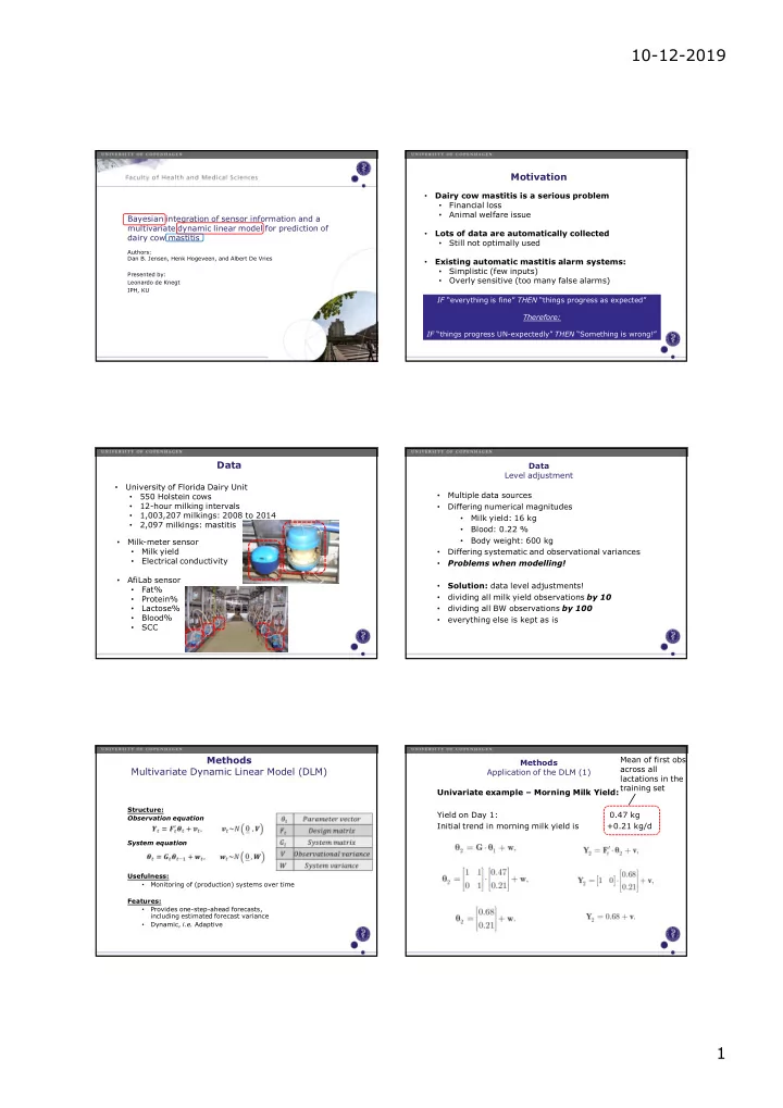
Bayesian integration of sensor information and a multivariate dynamic linear model for prediction of Lots of data are


  1. 10-12-2019 Motivation Dairy cow mastitis is a serious problem • Financial loss • Animal welfare issue Bayesian integration of sensor information and a • multivariate dynamic linear model for prediction of Lots of data are automatically collected dairy cow mastitis • Still not optimally used • Authors: Dan B. Jensen, Henk Hogeveen, and Albert De Vries Existing automatic mastitis alarm systems: • Simplistic (few inputs) Presented by: • Overly sensitive (too many false alarms) Leonardo de Knegt • IPH, KU IF “everything is fine” THEN “things progress as expected” Therefore: IF “things progress UN-expectedly” THEN “Something is wrong!” Data Data Level adjustment University of Florida Dairy Unit • Multiple data sources 550 Holstein cows • • 12-hour milking intervals Differing numerical magnitudes • • 1,003,207 milkings: 2008 to 2014 Milk yield: 16 kg • • 2,097 milkings: mastitis • Blood: 0.22 % • Body weight: 600 kg Milk-meter sensor • • Milk yield Differing systematic and observational variances • • Electrical conductivity Problems when modelling! • • AfiLab sensor • Solution: data level adjustments! Fat% • • dividing all milk yield observations by 10 Protein% • • Lactose% dividing all BW observations by 100 • • Blood% everything else is kept as is • • SCC • Methods Mean of first obs Methods across all Multivariate Dynamic Linear Model (DLM) Application of the DLM (1) lactations in the training set Univariate example – Morning Milk Yield: Structure: Yield on Day 1: 0.47 kg Observation equation Initial trend in morning milk yield is +0.21 kg/d System equation Usefulness: Monitoring of (production) systems over time • Features: Provides one-step-ahead forecasts, • including estimated forecast variance Dynamic, i.e. Adaptive • 1

  2. 10-12-2019 Matrix multiplication – simple example Matrix multiplication – simple example θ 1 The system θ 2 The design matrix G has a matrix F’ has a An element in the 0.47 structure which An element in the 0.68 structure which product is produces the product is separates the sum of the observable calculated as the calculated as the 0.21 0.21 previous values from the product of a row and product of a row and estimate with unobservable a column a column the expected trends, 1 1 F’ 1 0 0.68 0.68 trend on the producing a G yield row, when vector of the 0 1 0.21 multiplied with expected theta. observation Y t Methods Methods Application of the DLM (1) Application of the DLM (1) The multi-variate case – repeat for each variable: The multi-variate case – repeat for each variable: � � � � � � � � � � � � � � 1 � � � � � � � � � � � � � � 2 � � � � � � � � � � � � � � 3 F’ t � � � � � � � � � � � � � � � 4 � � � � � � � � � � � � � � 5 � � � � � � � � � � � � � � 6 � � � � � � � � � � � � � � 7 F’ t � � � Methods Methods Application of the DLM (1) Application of the DLM (1) The multi-variate case – repeat for each variable: The multi-variate case – repeat for each variable: 1,1 … 1,7 G t � � � Co-dependencies � � � � � � � � � � � � � � � � 1 between observable � � � � � � � � � � � � � � variables � � � � � � � � � � � � � � 2 7,1 … 7,7 � � � � � � � � � � � � � � � � � � � � � � � � � � � � 3 � � � � � � � � � � � � � � � � � � � � � � � � � � � � G t � 4 � � � � � � � � � � � � � � Co-dependencies � � � � � � � � � � � � � � 5 between observable � � � � � � � � � � � � � � and unobservable � � � � � � � � � � � � � � 6 (d) variables � � � � � � � � � � � � � � � � � � � � � � � � � � � � 7 � � � � � � � � � � � � � � 2

  3. 10-12-2019 CLASS QUESTIONS Q1: What is wrong with my milk yield model? Q2: What could be done to fix this problem? Learning the likelihoods Learning the likelihoods - sensor example The Different variables The possible High observations Middle-High The probability of making that Middle-Low observation, given Low that the cow has mastitis The probability of making that observation, given that the cow does not have mastitis Applying the likelihoods Applying the likelihoods MY CE F% P% L% B% SSC BW Prior(pos) = 0.5  p(Pos|Yield,Season) = 0.78 Prior probability of Mastitis: 5 % 16 % Prior(pos) = 0.05  p(Pos|Yield,Season) = 0.16 Observed ariable p(Observed |Pos) p(Observed |Neg) Mast. category Low 0.38 0.15 Middle-Low 0.25 0.34 Milk Yield Middle-High 0.23 0.36 High 0.14 0.15 Prev. Cold 0.53 0.66 Season Parity Seas. WIM Warm 0.47 0.34 M 3

  4. 10-12-2019 Performances Output examples Morning vs. Evening vs. Both AUC = 0.89 SE = 0.80 SP = 0.81 Concluding remarks Advantages: Good way of combining sensor and non-sensor data • Missing data can be easily handled • Needed improvements: Biologically meaningful trend functions • Better performance in the first two weeks of lactation • Perspectives: Alternatives to naive Bayesian classifyer • 4

Download Presentation
Download Policy: The content available on the website is offered to you 'AS IS' for your personal information and use only. It cannot be commercialized, licensed, or distributed on other websites without prior consent from the author. To download a presentation, simply click this link. If you encounter any difficulties during the download process, it's possible that the publisher has removed the file from their server.

Recommend


More recommend