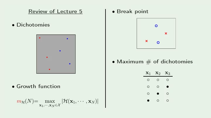
0.5 1 1.5 2 2.5 3 Maximum # of dihotomies Gro wth - PowerPoint PPT Presentation

PSfrag repla ements 0 0.5 1 1.5 2 Review of Le ture 5 Break p oint 2.5 3 3.5 Di hotomies 4 • 0.5 1 1.5 • 2 2.5 3 Maximum # of di hotomies • Gro wth fun tion x 1 x 2 x 3 ◦ ◦ ◦ • ◦ ◦ • ◦ • ◦ • ◦ ◦ m H ( N )= x 1 , ··· , x N ∈X |H ( x 1 , · · · , x N ) | max

Lea rning F rom Data Y aser S. Abu-Mostafa Califo rnia Institute of T e hnology Le ture 6 : Theo ry of Generalization Sp onso red b y Calte h's Provost O� e, E&AS Division, and IST Thursda y , Ap ril 19, 2012 •

Outline Pro of that m H ( N ) is p olynomial • Pro of that m H ( N ) an repla e M • Creato r: Y aser Abu-Mostafa - LFD Le ture 6 2/18 M � A L

Bounding m H ( N ) T o sho w: is p olynomial W e sho w: a p olynomial m H ( N ) m H ( N ) ≤ · · · ≤ · · · ≤ Key quantit y: : Maximum numb er of di hotomies on N p oints, with b reak p oint k B ( N, k ) Creato r: Y aser Abu-Mostafa - LFD Le ture 6 3/18 M � A L

Re ursive b ound on B ( N, k ) Consider the follo wing table: # of ro ws . . . . . . . . . . . . . . . . . . x 1 x 2 x N − 1 x N +1 +1 +1 +1 . . . − 1 +1 +1 − 1 . . . B ( N, k ) = α + 2 β S 1 α . . . . . . . . . . . . . . . +1 − 1 − 1 − 1 . . . − 1 +1 − 1 +1 . . . +1 − 1 +1 +1 . . . − 1 − 1 +1 +1 . . . S + β 2 . . . . . . . . . . . . . . . +1 − 1 +1 +1 . . . − 1 − 1 − 1 +1 . . . S 2 +1 − 1 +1 − 1 . . . − 1 − 1 +1 − 1 . . . Creato r: Y aser Abu-Mostafa - LFD Le ture 6 4/18 S − β 2 +1 − 1 +1 − 1 . . . − 1 − 1 − 1 − 1 . . . M � A L

Estimating α and β F o us on x 1 , x 2 , · · · , x N − 1 olumns: # of ro ws . . . . . . . . . . . . . . . . . . x 1 x 2 x N − 1 x N +1 +1 +1 +1 . . . − 1 +1 +1 − 1 . . . α + β ≤ B ( N − 1 , k ) S 1 α . . . . . . . . . . . . . . . +1 − 1 − 1 − 1 . . . − 1 +1 − 1 +1 . . . +1 − 1 +1 +1 . . . − 1 − 1 +1 +1 . . . S + β 2 . . . . . . . . . . . . . . . +1 − 1 +1 +1 . . . − 1 − 1 − 1 +1 . . . S 2 +1 − 1 +1 − 1 . . . − 1 − 1 +1 − 1 . . . Creato r: Y aser Abu-Mostafa - LFD Le ture 6 5/18 S − β 2 +1 − 1 +1 − 1 . . . − 1 − 1 − 1 − 1 . . . M � A L

Estimating β b y itself No w, fo us on the S 2 = S + ro ws: # of ro ws . . . . . . . . . . . . . . . 2 ∪ S − 2 . . . x 1 x 2 x N − 1 x N +1 +1 +1 +1 . . . − 1 +1 +1 − 1 . . . β ≤ B ( N − 1 , k − 1) S 1 α . . . . . . . . . . . . . . . +1 − 1 − 1 − 1 . . . − 1 +1 − 1 +1 . . . +1 − 1 +1 +1 . . . − 1 − 1 +1 +1 . . . S + β 2 . . . . . . . . . . . . . . . +1 − 1 +1 +1 . . . − 1 − 1 − 1 +1 . . . S 2 +1 − 1 +1 − 1 . . . − 1 − 1 +1 − 1 . . . Creato r: Y aser Abu-Mostafa - LFD Le ture 6 6/18 S − β 2 +1 − 1 +1 − 1 . . . − 1 − 1 − 1 − 1 . . . M � A L

Putting it together # of ro ws . . . . . . . . . . . . . . . B ( N, k ) = α + 2 β . . . x 1 x 2 x N − 1 x N +1 +1 +1 +1 . . . − 1 +1 +1 − 1 . . . α + β ≤ B ( N − 1 , k ) S 1 α . . . . . . . . . . . . . . . +1 − 1 − 1 − 1 . . . − 1 +1 − 1 +1 . . . β ≤ B ( N − 1 , k − 1) +1 − 1 +1 +1 . . . − 1 − 1 +1 +1 . . . S + β 2 . . . . . . . . . . . . . . . +1 − 1 +1 +1 . . . − 1 − 1 − 1 +1 . . . B ( N, k ) ≤ S 2 +1 − 1 +1 − 1 . . . − 1 − 1 +1 − 1 . . . Creato r: Y aser Abu-Mostafa - LFD Le ture 6 7/18 S − β 2 B ( N − 1 , k ) + B ( N − 1 , k − 1) +1 − 1 +1 − 1 . . . − 1 − 1 − 1 − 1 . . . M � A L

Numeri al omputation of B ( N, k ) b ound B ( N, k ) ≤ B ( N − 1 , k ) + B ( N − 1 , k − 1) k 1 2 3 4 5 6 . . top 1 1 2 2 2 2 2 . . 2 1 3 4 4 4 4 . . bottom 3 1 4 7 8 8 8 . . N 4 1 5 11 . . . . . . . . 5 1 6 : . 6 1 7 : . Creato r: Y aser Abu-Mostafa - LFD Le ture 6 8/18 : : : : . M � A L

Analyti solution fo r B ( N, k ) b ound B ( N, k ) ≤ B ( N − 1 , k ) + B ( N − 1 , k − 1) Theo rem: k 1 2 3 4 5 6 . . 1 1 2 2 2 2 2 . . 2 1 3 4 4 4 4 . . k − 1 � N � � B ( N, k ) ≤ 3 1 4 7 8 8 8 . . i top i =0 N 4 1 5 11 . . . . . . . . 1. Bounda ry onditions: easy 5 1 6 : . bottom 6 1 7 : . Creato r: Y aser Abu-Mostafa - LFD Le ture 6 9/18 : : : : . M � A L

2. The indu tion step top k − 1 k − 1 k − 2 � N � � N − 1 � � N − 1 � k−1 k � � � N−1 = + ? i i i i =0 i =0 i =0 N k − 1 � N − 1 � k − 1 � N − 1 � bottom � � = 1+ + i − 1 i i =1 i =1 k − 1 �� N − 1 � � N − 1 �� � = 1 + + i − 1 i i =1 k − 1 k − 1 � N � � N � � � = 1 + = Creato r: Y aser Abu-Mostafa - LFD Le ture 6 10/18 � i i i =1 i =0 M � A L

It is p olynomial! F o r a given H , the b reak p oint k is �xed k − 1 � N � � maximum p o w er is N k − 1 m H ( N ) ≤ i i =0 � �� � Creato r: Y aser Abu-Mostafa - LFD Le ture 6 11/18 M � A L

Three examples k − 1 � N � � is p ositive ra ys: (b reak p oint k = 2 ) i i =0 • H is p ositive intervals : (b reak p oint k = 3 ) m H ( N ) = N + 1 ≤ N + 1 • H is 2D p er eptrons : (b reak p oint k = 4 ) 2 N 2 + 1 2 N 2 + 1 m H ( N ) = 1 1 2 N + 1 ≤ 2 N + 1 Creato r: Y aser Abu-Mostafa - LFD Le ture 6 12/18 • H 6 N 3 + 5 1 m H ( N ) = ? ≤ 6 N + 1 M � A L

Outline Pro of that m H ( N ) is p olynomial • Pro of that m H ( N ) an repla e M • Creato r: Y aser Abu-Mostafa - LFD Le ture 6 13/18 M � A L

What w e w ant Instead of: P [ | E P in ( g ) − E out ( g ) | > ǫ ] ≤ 2 e − 2 ǫ 2 N M W e w ant: P [ | E P in ( g ) − E out ( g ) | > ǫ ] ≤ 2 m H ( N ) e − 2 ǫ 2 N Creato r: Y aser Abu-Mostafa - LFD Le ture 6 14/18 M � A L

Pi to rial p ro of Ho w do es m H ( N ) relate to overlaps? • What to do ab out E ? out • Putting it together • Creato r: Y aser Abu-Mostafa - LFD Le ture 6 15/18 M � A L

Hoeffding Inequality Union Bound VC Bound space of data sets . D Creato r: Y aser Abu-Mostafa - LFD Le ture 6 16/18 (a) (b) (c) M � A L

What to do ab out E out Hi E E (h) (h) out out E in (h) E ’ E Creato r: Y aser Abu-Mostafa - LFD Le ture 6 17/18 in (h) in (h) Hi M � A L

Putting it together Not quite: P [ | E P in ( g ) − E out ( g ) | > ǫ ] ≤ 2 m H ( N ) e − 2 ǫ 2 N but rather: P [ | E P in ( g ) − E out ( g ) | > ǫ ] ≤ 4 m H (2 N ) e − 1 8 ǫ 2 N The V apnik-Chervonenkis Inequalit y Creato r: Y aser Abu-Mostafa - LFD Le ture 6 18/18 M � A L