z i w w * b dz 0 Lecture 16, Slide 1 Buoyancy flux profile - PowerPoint PPT Presentation

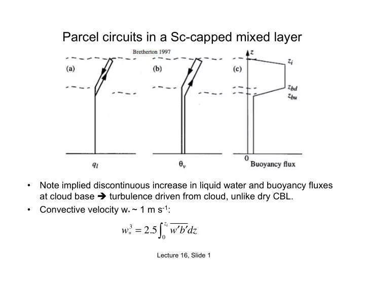
Parcel circuits in a Sc-capped mixed layer • Note implied discontinuous increase in liquid water and buoyancy fluxes at cloud base è turbulence driven from cloud, unlike dry CBL. • Convective velocity w * ~ 1 m s -1 : 3 = 2.5 ∫ z i w ′ ′ w * b dz 0 Lecture 16, Slide 1

Buoyancy flux profile in a Sc-capped mixed layer Solid: T v flux (buoyancy flux) Dotted: T vl flux Dashed: Scaled latent heat flux Buoyancy flux minimum just below cloud base. Buoyancy flux jump at cloud base is approx. proportional to LHF, with proportionality constant σ ~ 0.35. Bretherton and Wyant 1997, Fig. 4 Lecture 16, Slide 2

Sc MLM entrainment closure Nicholls-Turton (1986) entrainment closure Observational test with Fit to aircraft and lab obs and dry CBL SE Pacific Sc diurnal cycle 3 w e = A w * (Caldwell et al. 2005) A = 0.2(1 + a 2 E ), Δ b = g Δ T v T 0 z i Δ b , Evaporative enhancement: Less buoyant mixtures easier to entrain. NT enhancement factor E = Δ m / Δ T v a 2 = 15-60 è A = 0.5 - 5 in typical Sc T v ´ Δ T v 2 Δ m NT: Nicholls and Turton (1986) DL: Lilly (2002) 0 1 LL: Lewellen&Lewellen (2003) χ * ≈ 0.1 Entrained fraction χ Lecture 16, Slide 3

Profiles in a stratocumulus-capped mixed layer h + q t + W ( z ) E ( z ) B ( z ) T w z w e q l W ( z i ) z i ρ ′ w ′ q v P h ρ ′ w ′ q t z b F R h M q tM T Ms W (0) q s h s T s Fluxes State variables Lecture 16, Slide 4

MLM examples Steady-state solutions: Higher SST, lower divergence promote deeper mixed layer with thicker cloud. SST = 16 C, D = 4x10 -6 s -1 Cloud top Cloud base SST = 17 C, D = 3x10 -6 s -1 Schubert et al. 1979a, JAS Lecture 16, Slide 5

MLM response to a +2K SST jump Two timescales: Fast internal adjustment t b = z i / C T V ~ 0.5 day Slow inversion adjustment t i = D -1 ~ 3 days Schubert et al. 1979b JAS Lecture 16, Slide 6

Eddy velocity vs. flux-partitioning entrainment closures • Overall MLM evolution is not too sensitive to closure because the MLM adjusts w e to maintain energy balance in which entrainment warming roughly balances total BL radiative cooling (which mainly just cares about the cloud fraction). • Subcloud buoyancy fluxes are sensitive to the closure. In simulations of MLM evolution over a warming SST, NT (w*) closure predicts increasing negative subcloud buoyancy fluxes as the BL deepens, implying decoupling after 2.2 days. The flux-partitioning closure cannot do this. Lecture 16, Slide 7

MLM diurnal cycle Schubert 1976 JAS MLM prediction: cloud thickens during the day because of decreased entrainment, opposite to observations. The problem is that the mixed layer assumption breaks down during daytime . Lecture 16, Slide 8

Multiple mixed layer model Turton and Nicholls 1987 QJ Lecture 16, Slide 9