THE ORBITSPHERE - LATITUDINAL FLUX (also could be called azimuthal - PDF document

THE ORBITSPHERE - LATITUDINAL FLUX (also could be called ” azimuthal flux ”) As further exploration of the intricacies of the motions of charged sub- elements of the Orbitsphere, we here discuss the Latitudinal Flux of the Orbitsphere - that is - if we were to consider the Orbitsphere to be a globe with a North Pole (the point on the sphere obtained by moving from the nucleus in the direction of the Orbitsphere’s net angular momen- tum vector), a South Pole, an Equator, parallels of Latitude and circles of Longitude, we seek to calculate the amount of charge flowing along the 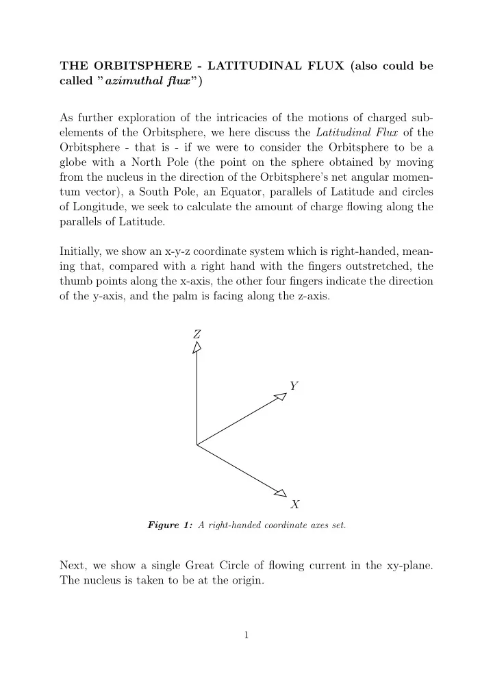parallels of Latitude. Initially, we show an x-y-z coordinate system which is right-handed, mean- ing that, compared with a right hand with the fingers outstretched, the thumb points along the x-axis, the other four fingers indicate the direction of the y-axis, and the palm is facing along the z-axis. Z Y X Figure 1: A right-handed coordinate axes set. Next, we show a single Great Circle of flowing current in the xy-plane. The nucleus is taken to be at the origin. 1

Z Y X Figure 2: Right-handed coordinate axes set with sin- gle Great Circle of current in xy-plane. This will be the ” equator ” of the Orbitsphere. Next, we perform Residue Rotation of this Great Circle about the y-axis and we obtain Figure 3. Z Y X Figure 3: An cylindrical Orbitsphere-like structure. The Filamentary Circle are in planes parallel to the xy-plane. The velocity of mass (charge) flow around each circle is given by v=a+bz where z is the z-coordinate of the Fila- mentary Circle. 2

Figure 4 is like Figure 3 except that the pitch is 30 o rather than 10 o . The image of Figure 4 is used to generate the Orbitsphere shown in Figure 5. Z Y X The velocity-transformed surface of the Figure 4: Orbitsphere-like structure of Figure 3. Z Y X Figure 5: Orbitsphere generated from Residue Rotation through 360 o about z-axis of the image of Figure 4 using pitch angle of 30 o . 3

Z Y X Figure 6: Some of the parallels of latitude are shown in blue, superposed over the pushed-in slinky of Figure 3. Figure 6 shows some of the parallels of latitude. The objective of the present exercise is to calculate, for the Orbitsphere, the amount of charge flowing along the respective parallels of latitude, that, is the ” Latitudinal Flux ”. The Orbitsphere is generated via residue rotation of the pushed-in slinky image of Figure 3. If we know the Latitudinal Flux for the pushed-in slinky, then the Latitudinal Flux for the Orbitsphere will be that for a single pushed-in slinky multiplied by the number of pushed-in slinky im- ages used to generate the Orbitsphere. Therefore, it is only necessary to calculate the Latitudinal Flux for the pushed-in slinky, which we would then multiply by an integer constant to find out the Latitudinal Flux for the whole Orbitsphere. Figure 7 shows the image of Figure 6 seen edge-on, looking along positive y-axis. We see that to obtain the Latitudinal Flux, it is necessary to first obtain the Latitudinal Flux for a single Great Circle, and then sum over the Great Circles which make up the pushed-in slinky image. 4

Z X Figure 7: Image as Figure 6 but seen looking from a distance in direction of positive-y axis. Next, we show the mathematical calculation to find the Latitudinal com- ponent of the current flowing in a single Great Circle. Z | � � OB | = 1 OB = b | � � OA | = 1 OA = a Y B A θ T O X 5

r = cos θ a + sin θ b (1) a = cos T i + sin T k (2) b = j (3)     cos T 0  + sin θ r = cos θ 0 1 (4)    sin T 0   cos θ cos T r = sin θ (5)   cos θ sin T   − sin θ cos T d r dθ = cos θ (6)   − sin θ sin T � d r � − sin θ cos T � � = (7) � cos θ dθ � xy � � � d r � � � = [sin 2 θ cos 2 T + cos 2 θ ] 1 / 2 � modulus = m = (8) � � � � dθ � � xy � z = cos θ sin T (9) z 2 sin 2 T = cos 2 θ (10) z 2 sin 2 T = sin 2 θ 1 − (11) 6

We have used a C++/OpenGL program to calculate the Latitudinal Flux according to equation (8). Figure 8, generated via this program, shows the pushed-in slinky image also with the angular momentum vectors for each Great Circle of flowing charge ( in quadrant for x < 0 , z > 0). To the right of this diagram, the Latitudinal Flux for each Great Circle is plotted. The Latitudinal Flux m for a point (x,y,z) on a Great Circle is calculated then plotted at the same z-displacement as the corresponding point on the Great Circle and with a horizontal displacement from the line segment AB proportional to m . Also, each Great Circle is plotted in a particular color, and the same color is used for the corresponding plot of Latitudinal Flux. Figure 8: Fan of Great Circles seen edge-on with corre- sponding plot of Latitudinal Flux for each (un-normalized) Great Circle. Angular momentum vectors for each Great Circle are also shown in quadrant x < 0 , z > 0 . To make Figure 8, it was assumed that all Great Circles of the pushed- in slinky had the same current flow. Hence the Great Circles are un- normalized, and performing the Residue Rotation about the z-axis of the pushed-in slinky would create an un-normalized orbitsphere ( one for which the Charge Density on the surface is non-uniform ). Recall that creation of a normalized Orbitsphere can be done by multiplying the current (and consequently the charge) in each Great Circle by the corresponding nor- malization factor referred to as the G-factor [2]. 7

The G-factor was derived [2] to refer to the tip of the Angular Momen- tum vector for each un-normalized Great Circle, the Angular Momentum vector being drawn from the origin. In Figure 8, assume that the angular momentum vectors all have length 1. The tips of these vectors then are located at ( x L ,0, z L ). The G-factor is defined in reference to z L and is given [2] by � G = z L − ( z L ) 2 (12) Use of this weighting factor G can be used to generate a uniform-density Orbitsphere, as has been shown in [2]. Figure 9 shows the G factor as a horizontal line segment of horizontal length proportional to G-factor, and at z-height same as corresponding tip of angular momentum vector. Also color of line segment representing G is same as color of corresponding angular momentum vector and Great Circle. Figure 9: G-factor of equation (12) . Next, we show the Latitudinal Flux for the respective Great Circles when the current/charge is multiplied by this G-factor (Figure 10). 8

Figure 10: Latitudinal Flux as horizontal distance from AB (as in Figure 8) but with multiplication by G-factor. In Figure 10, there is the red Great Circle in the yz-plane which has a G-factor of zero, and hence the corresponding Latitudinal Flux is zero, and so the respective plot of Latitudinal Flux is superposed upon the line segment AB ( horizontal distance from AB of point on plot is proportional to Latitudinal Flux ). Next, we increase the number of Great Circles used to make the plots. Figures 11 and 12 are for two separate fans of Great Circles, so that one can see the Latitudinal Flux plots better than if one were to just use a single fan of densely-packed Great Circles. 9

Figure 11: Latitudinal Flux plot as in Figure 10 but with number of Great Circles increased, and also angle of tilt of Great Circle from xy-plane ranges from 0 to 45 o . Figure 12: Latitudinal Flux plot as in Figure 10 but with number of Great Circles increased, and also angle of tilt of Great Circle from xy-plane ranges from 45 o to just under 90 o . 10

Now we have seen graphs of the Latitudinal Flux for the normalized Great Circles that make up the fan of Great Circles, the next step is to calculate the total Latitudinal Flux, summing over the Great Circles that enter the space between the planes (z=Z) and (z=Z+∆Z). To have the program do this, we use an Array Variable LatFdeltaz [] with array subscript from 0 to 499. The z-axis from z = 0 to z = r is divided into small segments, each segment corresponding to a particular subscript of the array variable LatFdeltaz []. When the normalized Latitudinal Flux is calculated for a particular subdivision of the Great Circle, the z-coordinate of this sub- division is matched to the corresponding subscript of the array variable, and the value of that particular LatFdeltaz [ subscript ] is increased by the normalized Latitudinal Flux value for the Great Circle subdivision. This summation process causes a discrete chunkiness to be introduced into the value for the total Latitudinal Flux due to the size of the Great Circle subdivisions, the plane angular separation between successive Great Cir- cles in the fan of Great Circles, and the division of the z-axis into 500 units. Figure 14 shows the normalized Total Latitudinal Flux for a fan of six Great Circles. The Great Circles in the xy and yz planes have a zero G- factor, and so it is only the four Great Circles at oblique angles to these planes which contribute to the Total Latitudinal Flux. As one can see, at the vertically-highest points of these four Great Circles the Total Lat- itudinal Flux function increases to a maximum. This is because at the vertically-highest point, all the charge in the Great Circle is flowing lati- tudinally. 11