Vibrational spectra of model Chromophores P. Giannozzi - PowerPoint PPT Presentation

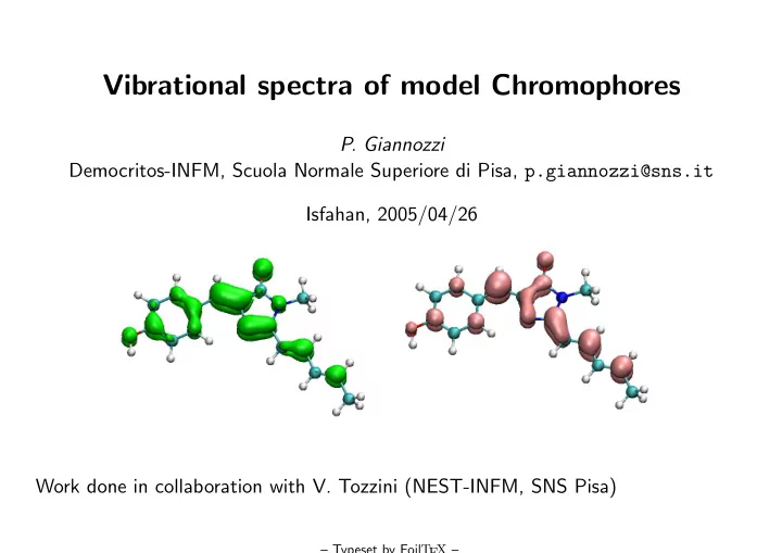
Vibrational spectra of model Chromophores P. Giannozzi Democritos-INFM, Scuola Normale Superiore di Pisa, p.giannozzi@sns.it Isfahan, 2005/04/26 Work done in collaboration with V. Tozzini (NEST-INFM, SNS Pisa) – Typeset by Foil T EX –

Vibrational Spectroscopy: experiment • Observation of vibrational modes: phonons in crystals, normal modes in molecules, is a powerful tool in materials characterization • Vibrational spectroscopy is a sensitive probe of the atomic structure and of the chemical bonding and thus of the electronic structure • Most frequently used experimental techniques: Infrared and Raman – both simple and effective Theoretical calculation of vibrational mode frequencies and intensities from first principles is very helpful in analyzing vibrational spectra

Vibrational frequencies: calculation Normal mode frequencies, ω , and displacement patterns, U α I for cartesian component α of atom I , are determined by the secular equation: � � � C αβ U β IJ − M I ω 2 δ IJ δ αβ J = 0 , J,β where C αβ IJ is the matrix of inter-atomic force constants (IFC), i.e. second derivatives of the energy with respect to atomic positions: IJ ≡ ∂ 2 E ( { R } ) = − ∂F α C αβ I I ∂R β ∂R β ∂R α J I where F I is the force acting on atom I at atomic position R I : F I = − ∂E ( { R } ) ∂ R I

Vibrational frequencies: calculation (2) Common methods – based on Density-functional Theory (DFT) – to calculate IFC’s: • Frozen-phonon technique: finite differentiation of forces • Density-functional Perturbation Theory (DFPT): direct calculation of second-order derivatives of the energy Alternative method: • Extract spectra from Molecular Dynamics runs, via the Fourier Transform of the velocity-velocity autocorrelation function

Calculation of Infrared and Raman Intensities Infrared (IR) Intensity: 2 � � � � � � Z ⋆αβ I U β � � I IR ( ν ) = I ( ν ) . � � � � α Iβ � � is proportional to the square of the induced dipole. The effective charges Z ⋆I is the polarization induced by an atomic displacement Non-resonant Raman intensities (Placzek approximation): 2 I Stokes ( ν ) ∝ ( ω L − ω ν ) 4 � � ∂χ αβ � � r αβ ( ν ) , r αβ ( ν ) = � � ∂u ( ν ) ω ν � � where χ is the electric polarizability, u ( ν ) is the normal mode coordinate along mode ν . Valid when ω L (incident laser frequency) << ω el (lowest electronic excitation energy)

Calculation of Infrared and Raman Intensities (2) The effective charge matrix is a second order derivative of the energy can be calculated using: • straightforward DFPT • the Berry’s phase approach The Raman tensor is a third-order derivative of the energy can be calculated using: • DFPT for χ + Frozen-phonon (finite differences) • DFPT using the (2 n + 1) theorem: the (2 n + 1) − th derivative of energy depends only on derivatives up to order n of the charge density. • DFPT + Second-order response to electric field • Finite electric fields + Frozen phonon

Density-Functional Theory Energy as a functional of the density n ( r ) : � E = T s [ n ( r )] + E H [ n ( r )] + E xc [ n ( r )] + n ( r ) V ( r ) d r is minimized by the ground-state charge density. Kohn-Sham equations for one-electron orbitals: h 2 H KS = − ¯ 2 m ∇ 2 + V H ( r ) + V xc ( r ) + V ( r ) ( H KS − ǫ i ) ψ i ( r ) = 0 , are solved self-consistently and the charge density is given by � | ψ i ( r ) | 2 n ( r ) = i (the sum is over occupied states)

Density-Functional Theory (2) Let us assume that the external potential depend on some parameter λ 2 λ 2 ∂ 2 V ( r ) V λ ( r ) ≃ V ( r ) + λ∂V ( r ) + 1 + ... ∂λ 2 ∂λ (all derivatives calculated at λ = 0 ) and expand the charge density 2 λ 2 ∂ 2 n ( r ) n λ ( r ) ≃ n ( r ) + λ∂n ( r ) + 1 + ... ∂λ 2 ∂λ and the energy functional accordingly: 2 λ 2 ∂ 2 E E λ ≃ E + λ∂E ∂λ + 1 ∂λ 2 + ... The first-order derivative ∂E/∂λ does not depend on any derivative of n ( r ) (Hellmann- Feynman theorem): ∂E n ( r ) ∂V ( r ) � ∂λ = ∂λ d r

Density-Functional Perturbation Theory (2) The second-order derivative ∂ 2 E/∂λ 2 can be written as a functional of ∂n/∂λ that must be minimized by the correct (ground-state) value for ∂n/∂λ . This results in a set of linear equations that determine ∂n/∂λ . At the minimum (ground state): � ∂V ( r ) ∂ 2 E n ( r ) ∂ 2 V ( r ) ∂n ( r ) � ∂λ 2 = ∂λ d r + d r ∂λ 2 ∂λ The result can be generalized to mixed derivatives: � ∂V ( r ) ∂ 2 E n ( r ) ∂ 2 V ( r ) ∂n ( r ) � ∂λ∂µ = ∂µ d r + ∂λ∂µ d r ∂λ (the order of derivatives can be exchanged)

Calculation of Linear Response The minimization of the second-order functional yields a set of equations: ( H − ǫ i ) ∂ψ i ( r ) ∂ψ j ∂V � + K ij ∂λ = − P c ∂λ | ψ i � ∂λ j where P c is the projector over unoccupied states, K ij is a nonlocal operator: e 2 � � � � ∂ψ j � | r − r ′ | + δv xc ( r ) j ( r ′ ) ∂ψ j ψ ∗ ∂λ ( r ′ ) d r ′ K ij ( r ) = 4 ψ i ( r ) ∂λ δn ( r ′ ) and the linear charge response: ∂n ( r ) i ( r ) ∂ψ i ( r ) � ψ ∗ = 2 Re ∂λ ∂λ i This scheme can be recast into the “traditional” self-consistent scheme

Application: Raman spectra of model chromophores The problem: characterization of the chromophore of proteins GFP (Green Fluorescent Proteins) and of DsRed (Red Fluorescent Protein). (b) (a) OH O Arg 96 H NH Gln 94 Thr 203 O O H Arg 96 NH2 NH2 Tyr 203 NH Gln 94 NH2 Tyr 203 O O N NH2 NH2 NH2 N O NH N Thr 203 N His 148 OH O H H N NH O O N O His 148 Asn 146 H H O H Thr 65 O H O H H H H O H O O O Ser 205 O H Asn 146 O H Thr 65 O H Glu 222 Ser 205 O O Glu 222 Scheme of the chromophore of GFP in the protein

Model chromophores O O CH 3 CH 3 N N N N OH OH CH 3 CH 3 Model chromophore of GFP: HBDI Model chromophore 1 of DsRed: HBMPI O CH 3 N N Model chromophore 2 of DsRed: HBMPDI OH CH 3

Raman Spectra for various Model Chromophores

Surface-Enhanced Raman Spectroscopy Results (HBDI Model Chromophore)

Surface-Enhanced Raman Spectroscopy Results (GFP protein)

Calculated Raman Intensities (HBDI Model Chromophore) GFP chromophore (all modes) (300−1200 cm−1 region) Raman Intensity (arb. units) 0 0 1000 2000 3000 300 500 700 900 1100 Frequency (cm−1) Frequency (cm−1) Placzek’s approximation (non resonant Raman), DFPT + Frozen-phonon

Some relevant normal mode patterns ν 5 ∼ 606cm − 1 Suppressed in the protein by geometrical constraints (protein backbone)

Some relevant normal mode patterns ν 8 ∼ 720cm − 1 Broadened and shifted in the protein

Some relevant normal mode patterns ν 11 ∼ 850cm − 1 Shifted at lower frequencies in the protein

Resonance Raman Raman spectra are often obtained in pre- resonant or resonant conditions, i.e. ω L < ω el or ω L ∼ ω el : The Placzek approximation does not hold. The expression for the Raman intensity is much more complicated, involving sums over electronic excited states: � � f | M α | e �� e | M β | i � � f | M β | e �� e | M α | i � � � σ αβ ( i → f ) ∝ + E e − E i − ¯ hω L − i Γ e E e − E f − ¯ hω L − i Γ e e ( M = electric dipole moment operator).

Calculation of pre-resonance Raman intensities In pre-resonance conditions, under various approximations: Born-Oppenheimer, harmonic ground state, Franck-Condon, the Raman intensity is proportional to the gradients of the excited-state potential energy surface(s): | M e | 2 ∂E e � σ ( i → f ) ∝ ∂u ( ν ) e calculated at the ground-state equilibrium positions Forces on ions on an excited state can be calculated using Time-Dependent DFT: F e = − ∂ ( E + ∆ E e ) ∂ R I where ∆ E e is the vertical excitation energy.

Calculation of (pre-)Resonance Raman intensities (2) Convenient algorithm • start a Molecular Dynamics run on the ground state, with initial velocities proportional to the forces calculated on the excited-state surface • extract the (mass-weighted) velocity-velocity autocorrelation function: � ∞ 1 e − iωt � √ f ( ω ) = m I � v I ( t ) · v I (0) � dt (1) 2 π −∞ I The resulting spectra mimic the pre-resonance Raman spectra, i.e. the height of the peaks is proportional to the Raman intensity, assuming that the main contribution comes from a specific excited-state

Results (preliminary) for HBMPDI Red: Raman intensity calculated for the S 2 excited state Green: as above for S 3 Blue lines: harmonic frequencies Inset: combined Raman intensity for S 2 and S 3

Conclusions • Calculation of vibrational frequencies and intensities from first principles is a useful tool in materials characterization • Both off-resonance and pre-resonance Raman intensities can be calculated from first principles with a manageable computational effort