Luminescence Spectroscopy Excitation is very rapid (10 - 15 s). - - PowerPoint PPT Presentation

139

Luminescence Spectroscopy

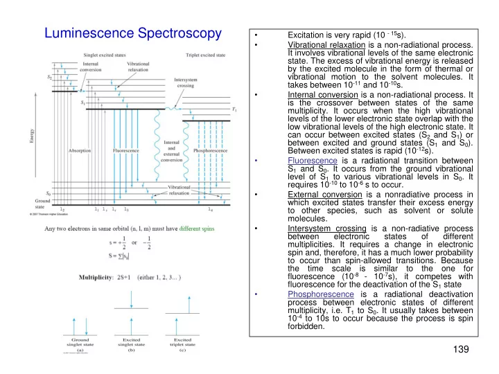
• Excitation is very rapid (10 - 15s).
• Vibrational relaxation is a non-radiational process.

It involves vibrational levels of the same electronic

• state. The excess of vibrational energy is released

by the excited molecule in the form of thermal or vibrational motion to the solvent molecules. It takes between 10-11 and 10-10s.

• Internal conversion is a non-radiational process. It

is the crossover between states of the same

• multiplicity. It occurs when the high vibrational

levels of the lower electronic state overlap with the low vibrational levels of the high electronic state. It can occur between excited states (S2 and S1) or between excited and ground states (S1 and S0). Between excited states is rapid (10-12s).

• Fluorescence is a radiational transition between

S1 and S0. It occurs from the ground vibrational level of S1 to various vibrational levels in S0. It requires 10-10 to 10-6 s to occur.

• External conversion is a nonradiative process in

which excited states transfer their excess energy to other species, such as solvent or solute molecules.

• Intersystem crossing is a non-radiative process

between electronic states

• f

different

• multiplicities. It requires a change in electronic

spin and, therefore, it has a much lower probability to occur than spin-allowed transitions. Because the time scale is similar to the one for fluorescence (10-8 - 10-7s), it competes with fluorescence for the deactivation of the S1 state

• Phosphorescence is a radiational deactivation

process between electronic states of different multiplicity, i.e. T1 to S0. It usually takes between 10-4 to 10s to occur because the process is spin forbidden.

140

Intensity of fluorescence (or phosphorescence) emission as a function of fluorophor (or phosphor) concentration

• The power of fluorescence (or phosphorescence) radiation (F or P)

is proportional to the radiant power of the excitation beam that is absorbed by the system: F = K’(P0 – P) (1)

• The transmittance of the sample is given by Beer’s law:

P/P0 = 10-ebc (2)

• Re-arranging Eq. 1:

F = K’ P0 (1 – P / P0)

• Substituting Eq. 2 above:

F = K’ (1 –10-ebc) (3)

• The exponential term in Eq. 3 can be expanded as a Maclaurin

series to: F = K’.P0.[2.303ebc – (2.303ebc)2 + (2.303ebc)3 - …] (4) 2! 3!

• For diluted solutions, i.e. 2.303ebc < 0.05, all of the subsequent

terms in the brackets become negligible with respect to the first, so: F = K’.P0.2.303ebc or F = 2.303.P0.K’.ebc (5)

• A plot of fluorescence (or phosphorescence) intensity as a function
• f concentration should be linear up to a certain concentration.
• Three are the main reasons for lack of linearity at high

concentrations: a) 2.303ebc > 0.05 b) self-quenching c) self-absorption

P0 P

LDR

Intensity Concentration

Detector

F

141

Fluorescence quantum yield

• The slope of the calibration curve is equal to

2.303.P0.K’.ebc.

• K’ is also known as the fluorescence

quantum yield (fF).

• The fluorescence quantum yield is the ratio

between the number of photons emitted as fluorescence and the number of photons absorbed: fF = # of fluorescence photons # of absorbed photons

• Fluorescence quantum yields may vary

between zero and unity: 0 < fF< 1 The higher the quantum yield, the stronger the fluorescence emission.

• In terms of rate constants, the fluorescence

quantum yield is expressed as follows: fF = kf kf + ki + kec + kic + kpd +kd

kf ki kec kic

• Consider a dilute solution of a fluorescent species A whose concentration is [A] (in mol.L-1). A

very short pulse of light at time 0 will bring a certain number of molecules A to the S1 excited state by absorption of photons: A + hν → A*

• The excited molecules then return to S0, either radiatively or non-radiatively, or undergo

intersystem crossing. As in classical kinetics, the rate of disappearance of excited molecules is expressed by the following differential equation:

• d[A*] / dt = (kf + knr) [A*]

knr = ki + kec + kic + kpd + kd are the rate constants of competing processes that ultimately reduce the intensity of fluorescence. k units = s-1.

142

Fluorescence lifetime

• Integration of equation:
• d[A*] / dt = (kf + knr) [A*]

yields the time evolution of the concentration of excited molecules [A*].

• Let [A*]0 be the concentration of excited

molecules at time 0 resulting from the pulse light

• excitation. Integration leads to:

[A*] = [A*]0 exp(-t / t)

where t is the lifetime of the excited state S1.

• The fluorescence lifetime is then given by:

t = 1 / kf + knr

• Typical fluorescence lifetimes are in the ns range.
• Typical phosphorescence lifetimes are in the ms

to s range.

• The fluorescence (or phosphorescence lifetime)

is the time needed for the concentration of excited molecules to decrease to 1/e of its

• riginal value.
• The fluorescence lifetime correlates to the

fluorescence quantum yield as follows: ff = kf. t

143

Excitation and emission spectra

• Excitation spectra appear in the same wavelength

region as absorption spectra.

• However, it is important to keep in mind that

absorption spectra are not the same as excitation spectra.

• Fluorescence

and phosphorescence spectra appear at longer wavelength regions than excitation spectra.

• Phosphorescence

spectra appear at longer wavelength regions than fluorescence spectra.

• In some cases, it is possible to observe vibrational

transitions in room-temperature fluorescence spectra. There are several parameters (many wavelengths and two lifetimes) for compound identification.

144

Fluorescence and Structure

• General rule: Most fluorescent compounds are
• aromatic. An increase in the extent of the p-electron

system (i.e. the degree of conjugation) leads to a shift

• f the absorption and fluorescence spectra to longer

wavelengths and an increase in the fluorescence quantum yield.

• Example:

Aromatic hydrocarbon Fluorescence Naphthalene ultraviolet Anthracene blue Naphthacene green Pentacene red

• The lowest-lying transitions of aromatic hydrocarbons

are of the p→p* type, which are characterized by high molar absorption coefficients and relatively high quantum fluorescence quantum yields.

No fluorescence Fluorescence

145

• The

effect

• f

substituents

• n

the fluorescence characteristics of aromatic hydrocarbons varies with the type of substituent.

• Heavy atoms: the presence of heavy atoms

(e.g. Br, I, etc.) results in fluorescence quenching (internal heavy atom effect) because of the increase probability of intersystem crossing (ISC).

• Electron- donating :
• OH, -OR, -NH2, -NHR, -NR2

This type of substituent generally induces and increase in the molar absorption coefficient and a shift in both absorption and fluorescence spectra.

• Electron-withdrawing substituents:

carbonyl and nitro-compounds Carbonyl groups: There is no “general rule”. Their effect depends

• n the position of the substituent

group in the aromatic ring. Nitro groups: No detectable fluorescence.

Substituted Aromatic Hydrocarbons

146

pH of solution Additional resonance forms lead to a more stable first excited state Rigidity Rigidity usually enhances fluorescence emission

147

Quenching

• Quenching: nonradiative energy transfer from an

excited species to other molecules.

• Quenching results in deactivation of S1 without

the emission of radiation causing a decrease in fluorescence intensity.

• Types of quenching: dynamic, static and others.
• Dynamic quenching: or collisional quenching

requires contact between the excited species and the quenching agent.

• Dynamic quenching is a diffusion controlled
• process. As such, its rate depends on the

temperature and viscosity of the sample.

• High temperatures and low viscosity promote

dynamic quenching.

• For dynamic quenching with a single quencher,

the Stern-Volmer expression is valid: F0/F = 1 + Kq[Q] Where F0 and F are the fluorescence intensities in the absence and the presence of quencher, respectively. [Q] is the concentration

• f

quencher (mols.L-1) and Kq is the Stern-Volmer quenching constant.

• The Stern-Volmer constant is defined as:

Kq = kq / kf + ki + kic where kq is the rate constant for the quenching process (diffusion controlled).

• Static Quenching: the quencher and the

fluorophor in the ground state form a complex. The complex is no fluorescent (dark complex).

• The Stern-Volmer equation is still valid but Kq in

this case is the equilibrium constant for complex formation: A + Q <=> AQ.

• In static quenching, the fluorescence lifetime of

the fluorophor is not affected. In dynamic quenching, the fluorescence lifetime of the fluorophor is affected. So, lifetime can be used to distinguish between dynamic and static quenching. Fluorescence quenching of quinine sulfate as a function of chloride concentration Oxygen sensors O2 is paramagnetic, i.e. its natural electronic configuration is the triplet state. When O2 interacts with the fluorophor, it promotes conversion and deactivation of excited fluorophor molecules. Upon interaction, O2 goes into the singlet state (diamagnetic).

148

Instrumentation

Typical spectrofluorometer (or spectrofluuorimeter) configuration Recording excitation and emission spectra Recording synchronous fluorescence spectra

149

Spectrofluorimeter capable to correct for source wavelength dependence Spectrofluorimeter with the ability to record total luminescence

150

Measuring phosphorescence

• Using a spectrofluorimeter with a continuous

excitation source: be careful with fluorescence and second order emission!

• Rotating-can phosphoroscope: “good-old” approach

to discriminate against fluorescence.

• A. True representation
• B. Approximate representation

te = exposure time; td = shutter delay time; tt = shutter transit time; tC = time for one cycle of excitation and observation; tE = te + tt; tD = td + tt

• Spectrofluorimeters with a pulsed source: employ a gated PMT for

fluorescence discrimination. Excitation source on => PMT off = fluorescence decays Excitation source off => PMT on – phosphorescence measurement

151

Introduction to Chromatographic Separations

• Analysis of complex samples usually involves

previous separation prior to compound determination.

• Two

main separation methods based

• n

instrumentation are available: Chromatography Electrophoresis

• Chromatography is based on the interaction of

chemical species with a mobile phase (MP) and a stationary phase (SP).

• The MP and the SP are immiscible.
• The sample is transported by the MP. The

interaction of species with the MP and the SP separates chemical species in zones or bands.

• The relative chemical affinity of chemical species

with the MP and the SP dictates the time the species remain in the SP.

• Two general types of chromatographic techniques

exist:

• Planar: flat SP, MP moves through capillary action
• r gravity
• Column: tube of SP, MP moves through gravity or

pressure.

SP Detector

MP + sample

152

Classification of Chromatographic Methods

• Chromatographic methods can be classified
• n the type of MP and SP and the kinds of

equilibrium involved in the transfer of solutes between phases: Column 1: Type of MP Column 2: Type of MP and SP Column 3: SP Column 4: Type of equilibrium Concentration profiles of solute bands A and B at two different times in their migration down the column.

153

Migration Rates of Solutes

• Two-component chromatogram illustrating two

methods for improving separation:

• (a) Original chromatogram with overlapping

peaks; (b) improvement brought about an increase in band separation; (c) improvement brought about by a decrease in the widths.

Distribution constant or partition ratio or partition coefficient: It describes the partition equilibrium of an analyte between the SP and the MP.

If K = Kc and SP = S and MP = M Kc = cS / CM = nS / VS nM / VM Where VS and VM are the volumes of the two phases and nS and nM are the moles of A in SP and MP, respectively.

154

Retention Time

• Retention time is a measured quantity.
• From the figure:

tM = time it takes a non-retained species (MP) to travel through the column = dead or void time. tR = retention time of analyte. The analyte has been retained because it spends a time tS in the SP. The retention time is then given by: tR = tS + tM

• The average migration rate (cm/s) of the

solute through the column is: Where L is the length of the column.

• The average linear velocity of the MP

molecules is:

155

Relationship Between Retention Time and Distribution Constant The Rate of Solute Migration: The Retention Factor

Where VS and VM are the volumes of SP and MP in the column. Knowing that: An equation can be derived to obtain KC of A (KA) as a function of experimental parameters.

=>

Retention factor = capacity factor = kA = k’A. However: k’A ≠ KC or k’A ≠ KA

=>

156

• The selectivity factor can be measured

from the chromatogram.

• Selectivity factors are always greater

than unity, so B should be always the compound with higher affinity by the SP.

• Selectivity

factors are useful parameters to calculate the resolving power of a column. Band Broadening and Column Efficiency

• The “shape” of an analyte zone eluting

from a chromatographic column follows a Gaussian profile.

• Some molecules travel faster than the
• average. The time it takes them to reach

the detector is: tR – Dt.

• Some molecules travel slower than the

average molecule. The time it takes them to reach the detector is: tR + Dt

• So, the Gaussian provides an average

retention time (most frequent time) and a time interval for the total elution of an analyte from the column.

• The magnitude of Dt depends on the

width of the peak.

157

• Considering that:

v_ = L / tR => L = v_ x

• r

L ± DL = v_ x [tR ± Dt]

• The equation above correlates chromatographic

peaks with Gaussian profiles to the length of the column.

• Both Dt and DL correspond to the standard

deviation of a Gaussian peak: Dt ≡ DL ≡ s

• If s = Dt, s units are in minutes. If s = DL, s units

are in cm.

• The width of a peak is a measure of the

efficiency of a column. The narrower the peak, the more efficient is the column. =>

• The efficiencies of chromatographic columns

can be compared in terms of number of theoretical plates .

158

The Plate Theory

• The plate theory supposes that the chromatographic

column contains a large number of separate layers, called theoretical plates.

• Separate equilibrations of the sample between the

stationary and mobile phase occur in these "plates".

• The analyte moves down the column by transfer of

equilibrated mobile phase from one plate to the next.

• It is important to remember that theoretical plates

do not really exist. They are a figment of the imagination that helps us to understand the processes at work in the column.

• As previously mentioned, theoretical plates also serve

as a figure of merit to measuring column efficiency, either by stating the number of theoretical plates in a column (N) or by stating the plate height (H); i.e. the Height Equivalent to a Theoretical Plate.

• The number of theoretical plates is given by:

N = L / H

• If the length of the column is L, then the HETP is:

H = s2 / L

• Note:
• For columns with the same

length (same L): The smaller the H, the narrower the peak. The smaller the H, the larger the number of plates. => column efficiency is favored by small H and large N.

• It is always possible to using a

longer column to improve separation efficiency.

159

Experimental Evaluation of H and N

• Calling s in time units (minutes or seconds) as t:

=> s / t = cm / s

• Considering that: v_ = L / tR = cm /s
• We can write:

L / tR = s / t

• r

t = s = s L / tR v_

• If the chromatographic peak is Gaussian,

approximately 96% of its area is included within ± 2s. This area corresponds to the area between the two tangents on the two sides of the chromatographic peak.

• The width of the peak at its base (W) is then

equal to: W = 4t in time units

• r

W = 4s in length units.

• Substituting t = W / 4 in the equation above we obtain:

s = LW / 4tR

• Substituting s = W / 4 in the same equation we obtain:

t = WtR / 4L

• Substituting s = LW / 4tR in the HEPT equation:

H = LW2 / 16tR2

• Substitution of this equation in N gives:

N = 16 (tR / W)2

• These two equations allow one to estimate H and N

from experimental parameters.

• If one considers the peak of the width at the half

maximum (W1/2): N = 5.54 (tR / W1/2)2

In comparing columns, N and H should be obtained with the same compound!

160

Kinetic Variables Affecting Column Efficiency

• The plate theory provides two figures of merit

(N and H) for comparing column efficiency but it does not explain band broadening.

• Table 26-2 provides the variables that affect

band broadening in a chromatographic column and, therefore, affect column efficiency.

• The effect of these variables in column

efficiency is best explained by the theory of band broadening. This theory is best represented by the van Deemter equation: H = A + B / u+ CS . u + CM . U where H is in cm and u is the velocity of the mobile phase in cm.s-1. The other terms are explained in Table 26-3.

• Table 26-3:

f(k) and f’(k) are functions of k l and g are constants that depend on the quality of the packing. B is the coefficient of longitudinal diffusion. CS and CM are coefficients of mass transfer in stationary and mobile phase, respectively.

• Before we try to understand the meaning of the

van Deemter equation, a better understanding

• f chromatographic columns is needed.

161

Some Characteristics of Gas Chromatography (GC) Columns

• Two general types

=> Open Tubular Columns (OTC) or Capillary Columns => Packed Columns

• OTC:

=> Wall Coated Open Tubular (WCOT) Columns => Support Coated Open Tubular (SCOT) Columns => The most common inner diameters for capillary tubes are 0.32 and 0.25mm.

• Packed Columns:

=> Glass tubes with 2 to 4mm inner diameter. => Packed with a uniform, finely divided packing material of solid support, coated with a thin layer (005 to 1mm) of liquid stationary phase.

• Solid Support Material in OTC and Packed

Columns Diatomaceous Earth: “skeletons of species

• f single-celled plants that once inhabited

ancient lakes and seas”.

162

Some Characteristics of HPLC Columns

• Only packed columns are used in

HPLC.

• Current packing consists of porous

micro-particles with diameters ranging from 3 to 10mm.

• The particles are composed of silica,

alumina, or an ion-exchange resin.

• Silica particles are the most common.
• Thin organic films are chemically or

physically bonded to the silica particles.

• The chemical nature of the thin
• rganic film determines the type of

chromatography.

SP for normal-phase chromatography SP for partition chromatography Typical micro- particle

163

Another Look at the van Deemter Equation

• H = A + B/u + CSu + CMu
• The multi-path term A or Eddy-Diffusion:

=> This term accounts for the multitude of pathways by which a molecule (or ion) can find its way through a packed column.

• A = 2ldp

where: l is a geometrical factor that depends on the shape

• f the particle: 1 ≤ l ≤ 2.

dp is the diameter of the particle.  Using packing with spherical particles

• f

small diameters should reduce eddy -diffusion.

Injection Detector

164

• The Longitudinal Diffusion Term B/u:
• Longitudinal diffusion is the migration of solute from

the concentrated center of the band to the more diluted regions on either side of the analyte zone.

• B/u = 2gDM/u

where: g is a constant that depends on the nature

• f the packing and it varies from 0.6 ≤ g ≤

0.8. DM is the diffusion coefficient in the mobile

• phase. DM a T / m, where T is the

temperature and m is the viscosity of the mobile phase.

• As u → infinite, B/u → zero. So, the contribution of

longitudinal diffusion in the total plate height is only significant at low MP flow rates.

• Its contribution is potentially more significant in GC

than HPLC because of the relatively high column temperatures and low MP viscosity (gas).

Initial band Diffusion of the band with time The initial part of the curve is predominantly due to the B/u term. Because the term B/u in GC is larger than HPLC, the overall H in GC is about 10x the overall H in HPLC.

165

• The Stationary-Phase Mass Transfer Term CSu:
• CS = mass transfer coefficient in the SP.

CS a df2 / DS where df is the thickness of the SP film and DS is the diffusion coefficient in the SP. => Thin-film SP and low viscosity SP (large DS) provide low mass transfer coefficients in the SP and improve column efficiency.

• The Mobile-Phase Mass Transfer Term CMu:
• CM = mass transfer coefficient in the MP.

CM a dp2 / DM where dp is the diameter of packing particles and DM is the diffusion coefficient in the MP.

• The contribution of mass transfer in the SP and MP on the
• verall late height depends on the flow velocity of the mobile
• phase. Both phenomena play a predominant role at high MP

flow rates.

Liquid SP coated on solid support Cartoon with example of SP mass-transfer in a liquid SP: different degrees of penetration

• f analyte molecules in the liquid layer of SP

lead to band-broadening Porous in silica particle Cartoon with example of MP mass- transfer: stagnant pools of MP retained in the porous of silica particles lead to band- broadening.

166

Summary of Methods for Reducing Band Broadening

• Packed Columns:
• Most important parameter that affects band

broadening is the particle diameter.

• If the SP is liquid, the thickness of the SP is

the most important parameter.

• Capillary Columns:
• No packing, so there is no Eddy-diffusion
• term. Most important parameter that affects

band broadening is the diameter of the capillary.

• Gaseous MP (GC):

The rate of longitudinal diffusion can be reduced by lowering the temperature and thus the diffusion coefficient.

• The effect of temperature is mainly noted at

low flow rate velocities where the term B/u is significant.

• Temperature has little effect on HPLC.

Effect of particle diameter in GC Effect of particle diameter in HPLC Note: m = mm

167

Optimization of Column Performance

• Optimization experiments are aimed at

either reducing zone broadening or altering relative migration rates of components.

• The time it takes for chromatographic

analysis is also an important parameter that should be optimized without compromising chromatographic resolution.

• Column Resolution:
• It is a quantitative measure of the ability of

the column to separate two analytes.

• It can be obtained from the chromatogram

with the equation:

• In terms of retention factors kA and kB for the

two solutes, the selectivity factor and the number of theoretical plates of the column:

• From the last equation we can obtain the

number of theoretical plates needed to achieve a given resolution:

168

• For compounds with similar capacity factors,

i.e. kA ≈ kB:

• The time it takes to achieve a separation

can be predicted with the formula:

Where k = kA + kB / 2

169

The General Elution Problem

• The general elution problem occurs in the

separation of mixtures containing compounds with widely different distribution constants.

• The best solution to the general elution

problem is to optimize eluting conditions for each compound during the chromatographic run.

• In HPLC, this is best accomplished by

changing the composition of the mobile phase (Gradient Elution Chromatography).

• In GC, this is best accomplished by changing

the temperature of the column during the chromatographic run.

170

Qualitative and Quantitative Analysis in GC and HPLC

• Both are done with the help of standards.
• Qualitative analysis, i.e. compound identification is done

via retention time. The retention time from the pure standard is compared to the retention time of the analyte in the sample. Note: retention times are experimental parameters and as such are prone to standard deviation.

• Quantitative analysis is done via the calibration curve

method (or external standard method) or the internal standard method.

• Calibration curve or external standard method: the

procedure is the same as usual. The calibration curve can be built plotting the peak height or the peak area versus standard concentration. The same volume of sample was injected in each case, but “Sample B ” has a much smaller peak. Since the tR at the apex of both peaks is 2.85 minutes, this indicates that they are both the same compound, (in this example, acrylamide (ID)). The “Area” under the peak (“ Peak Area Count ”) indicates the concentration of the compound. This area value is calculated by the Computer Data Station. Notice the area under the “Sample A” peak is much larger. In this example, “Sample A” has 10 times the area of “Sample B”. Therefore, “Sample A” has 10 times the concentration, (10 picograms) as much acrylamide as “Sample B”, (1 picogram). Note, there is another peak, (not identified), that comes out at 1.8 min. in both samples. Since the area counts for both “samples” are about the same, it has the same concentration in both samples.

171

Internal Standards

• An internal standard is a known amount of a

compound that is added to the unknown.

• The signal from analyte is compared to the

signal from the standard to find out how much analyte is present.

• This method compensates for instrumental

response that varies slightly from run to run and deteriorates reproducibility considerably.

• This is the case of mobile phase flow rate

variations in chromatographic analysis.

• Internal standards are also desirable in

cases where the possibility of loosing sample during analysis exists. This is the case

• f

sample separation in the chromatographic column.

• The internal standard should be chosen

according to the analyte. Their chemical behavior with regards to the SP and MP should be similar.

• How to use an internal standard?: a mixture

with the same known amount of standard and analyte is prepared to measure the relative response of the detector for the two species.

• The factor (F) is obtained from the relative

response of the detector.

• Once the relative response of the detector has

been found, the analyte concentration is calculated according to the formula:

Area of analyte signal = F x Area of standard signal Concentration of analyte Concentration of standard A known amount of standard is added to the unknown

• X. The relative response is measured to obtain the

detector’s response factor “F”.

172

Example of Internal Standards

• In a preliminary experiment, a solution

containing 0.0837M X and 0.066M S gave peak areas of AX = 423 and AS = 347. Note that areas are measured in arbitrary units by the instrument’s computer. To analyze the unknown, 10.0mL of 0.146M S were added to 10.0mL of unknown, and the mixture was diluted to 25.0mL in a volumetric flask. This mixture gave a chromatogram with peak areas AX = 553 and AS = 582. Find the concentration of X in the unknown.

• First use the standard mixture to find the

response factor: AX / [x] = F x {AS / [S]} Standard mixture: 423 / 0.0837 = F {347 / 0.0666} => F = 0.9700

• In the mixture of unknown plus standard, the

concentration of S is: [S] = (0.146M)(10.0mL / 25.0mL) = 0.0584M where: 10.0mL / 25.0mL is the dilution factor

• Using the known response factor and S

concentration of the diluted sample in the equation above: 553 / [X] = 0.9700 (582 / 0.0584) =>[X] = 0.05721M

173

Liquid Chromatography

Size exclusion or gel: polystyrene-divinylbenzene Silica with various porous sizes

174

Instrumentation

175

Pumping Systems

• Pumping systems that allow to change the

MP composition during the chromatographic run provide better separation of compounds with wide range of k’ factors.

176

Detectors

UV-VIS absorption cell for HPLC