Using nonlinear regression models for reconstructing Holocene - PowerPoint PPT Presentation

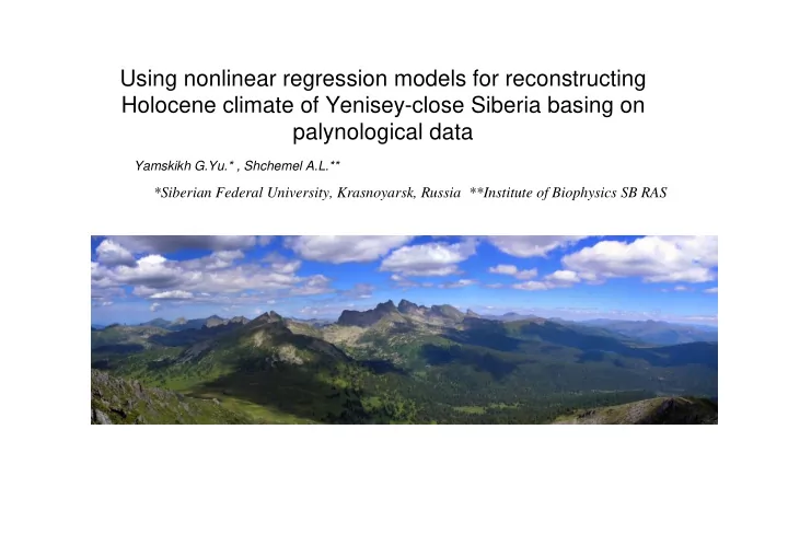
Using nonlinear regression models for reconstructing Holocene climate of Yenisey-close Siberia basing on palynological data Yamskikh G.Yu.* , Shchemel A.L.** *Siberian Federal University, Krasnoyarsk, Russia **Institute of Biophysics SB RAS

100% 90% 80% Spores 70% Grass and 60% low shrub 50% pollen 40% Trees and 30% shrubs 20% pollen 10% 0% 1 2 3 4 5 6 7 8 9 10 11 Ephedra Ericacea е 100% Poaceae Cyperaceae Artemisia Asteraceae Cichoriaceae Chenopodiaceae 80% Brassicaceae Saxifragaceae Fabaceae Liliaceae Iridaceae Euphorbiaceae 60% Ranunculaceae Thalictrum Caryophyllaceae Polygonaceae Violaceae Pyrolaceae 40% Rosaceae Onagraceae Geraniaceae Apiaceae Caprifoliaceae Valerianaceae 20% Rubiaceae Polemoniaceae Boraginaceae Campanulaceae 0% Nymphaeaceae Alismataceae Potamogetonaceae Sparganiaceae 1 2 3 4 5 6 7 8 9 10 11 Разнотравье Typhaceae 100% Salix Alnus 80% Dus с hekia fruticosa Betula sp. Betula sect. Albae 60% Betula sect. Nanae 40% Pinus sp. Pinus sylv estris Pinus sibirica 20% Picea obovata Abies sibirica 0% 1 2 3 4 5 6 7 8 9 10 11 Larix Riccia 100% Polipodiophyta 90% 80% Cryptogramma sp. 70% Aspleniaceae 60% Botrychium sp. 50% 40% Equisetaceae 30% Selaginella sanguinolenta 20% Selaginella sibirica 10% Selaginella selaginoides 0% 1 2 3 4 5 6 7 8 9 10 11 Lycopodium sp. Typical structure of spore-pollen spectrum Location of different types of sedimental probes and weather stations

Regional level of paleogeographical forecasts and correlation is not well developed yet. However they are very important for the understanding of mechanisms of global changes. Intracontinental territories have specific mechanisms of landscape formation. Paleoclimatic reconstructions for these areas are based on mathematical simulation. Major point of such simulation is quantitative interpretation of interdependence between vegetation and climatic changes. It is almost always impossible to make correct interpretations without correlations between spore-pollen data from sediments and recent samples. This is considered to be a reliable criteria for correlations between modern and past climate and vegetation. Paleoclimate and vegetation reconstructions in the intracontinental areas of Yenisei Siberia are specific because of the variability of factors which form spore-pollen spectra. Among them are atmosphere circulation and mountain-intermountain relief. These features determine peculiarities of climate differentiation and vegetation distribution. Specific group of landscapes are forming in the depressions - intermountain depression landscapes. Considering complexity of natural processes this group of landscapes can be compared with mountain areas. Correlation analysis was used at the initial stages of investigation. This allowed to estimate pare correlation coefficients between recent spore-pollen spectra and modern climate characteristics. Major aim of these analyses is revealing reguliarities between specific modern climate characteristics and spore-pollen spectra. Aiming to do that 794 recent samples from all the major genetic types of sediments from different landscapes were analyzed. Recent (surface) samples were divided into the eleven landscape zones and subzones. Their distribution among landscape zones and sediments is presented at upper-left figure. These samples were correlated with fourteen climate elements. Meteorological data were compiled from 95 meteorological stations. Each spore-pollen spectrum is characterized by 70 components. Maximal possible quantity of spectrum components –70 of initially 83 were used for investigation. Only rare elements were rejected. Each sample were correlated by 14 climate elements. Major aim is construction of universal model for intracontinental areas. That is why absolute height (Alt), geographical latitude (Lat) and geographical longitude (Long) were included in the models as factors. Then a nonlinear model which utilizes equation of a following form was built:

Size I ∑ ∑ = ∆ + sin( ϕ + f C u x ) at a a as si it = = 1 1 s i where a is an element of climate, s is a row of a matrix of model’s coefficient, i is a number of component of a sporo-pollen specter, t is a number of sample component, Size is a number of rows of matrix of the model, I is the quantity of the components of sporo-pollen specters, x is the value of the i -th element of the t -th spectre, u is a coefficient from the matrix, C is the coefficient used for normalization of each component of climate, f is a climate’s component, Δ are coefficients used to centralize f , are phase coefficients. To find coefficient of model we used constrained variant of Quazi-Newton optimization while norm was quadratic. Chosen form of dependences allowed calculate derivates very fast even when coefficients were quite a number and also perform regularization constraint fast as well. × ∑ si ≤ ≤ ϕ ≤ π 2 2 C u P 0 2 , s s , i where P is a chosen level of smoothness. ∑ 2 u s Such form allows to easily determine relevance of the input parameters: = s A ∑ i 2 u si s , i The same equations were used as discriminating functions to provide nonlinear classification of vegetation zones. So, we have got 14 equations to calculate each element of climate basing on spore-pollen spectrum, and 11 discriminating functions for classification vegetation zones.

Average Average temperature temperature Humidity Humidity Precipitation, mm Precipitation, mm temperature, º С temperature, º С Climate element Climate element Duration Duration Sum Sum Mean Mean of period of period of of July July January January annual annual without without active active temper temper severe severe tempe tempe April, April, ature, º ature, º Warm Warm Cold Cold frost, frost, rature rature Absolute, Absolute, Relative, Relative, Annua Annua Warm Warm Cold Cold May, May, Coefficient Coefficient С С >10 º C >10 º C Simulation’s accuracy Simulation’s accuracy period period Period Period days days mbar mbar % % l sum l sum period period period period June June of aridness of aridness Correlation coefficient Correlation coefficient 0.97 0.97 0.99 0.99 0.99 0.99 0.99 0.99 0.99 0.99 0.85 0.85 0.98 0.98 0.99 0.99 0.85 0.85 0.96 0.96 0.93 0.93 0.94 0.94 0.94 0.94 0.83 0.83 Mean square error Mean square error 0.014 0.014 0.027 0.027 0.011 0.011 0.019 0.019 0.012 0.012 0.31 0.31 2.26 2.26 0.0003 0.0003 0.085 0.085 2.07 2.07 1.46 1.46 1.29 1.29 0.58 0.58 0.009 0.009 Absolute mean error, % Absolute mean error, % 1.51 1.51 2.66 2.66 2.88 2.88 2.45 2.45 13.07 13.07 5.26 5.26 2.99 2.99 1.42 1.42 1.97 1.97 7.00 7.00 6.83 6.83 13.36 13.36 6.08 6.08 11.52 11.52 period without frost, days Diphasiastrum complanatum О б щ и й со с тав Precipitation, mm mean mean Humidity Coefficient of aridness 0 С 0 С п ы л ьцы temperature temperature, Возраст С 14 , лет назад Type of vegetation Palinological zone 0 С Duschekia fruticosa temperatures>10 и сп о р Betula sect. Nanae April, May, June , % Holocene period Betula sect. Albae Annual average 0 С Absolute, mbar Caryophyllaceae Chenopodiaceae temperature, Sum of active Lycopodium sp. Pinus sylvestris Ranunculaceae Polypodiophyta Warm period Warm period Стратиграфия Annual total Picea obovata Pinus sibirica Cichoriaceae Cold period Duration of Relative, % Cold period Abies sibirica Polygonaceae Equisetaceae Ericaceae Brassicaceae разнотравье Глубина , м Cyperaceae Thalictrum Asteraceae Typhaceae Sphagnum Rubiaceae Artemisia Apiaceae January Poaceae Bryales Larix July Salix 14 17 20 -26 -21 -16 8 9,5 10 -20 -15 -10 -3 -1 1 70 100 130 1200 1600 2000 5 6 7 65 70 75 400 600 800 300 450 600 0 100 200 100 200 300 1 1,5 2 5 1 0 1 01 0 5 0 5 0 2 5 1 0 2 0 5 0 2 0 2 0 1 0 1 0 1 01 0 1 0 1 0 5 0 1 0 1 0 5 5 0 5 0 2 0 5 5 5 0 5 0 20 4 0 6 0 8 0 10 0 IX 2 5 0± 5 0 SA VIII Г И Н 3 0 ,5 -42 5 2 VII 10 7 0± 1 0 0 Г И Н -42 7 9 SA 2 1 ,0 SA VI 1 2 75 0 ± 50 Г И Н -42 8 4 SB V 3 1 ,5 IV III 2 ,0 3 20 0 ± 90 SB 2 Г И Н -42 7 7 II I