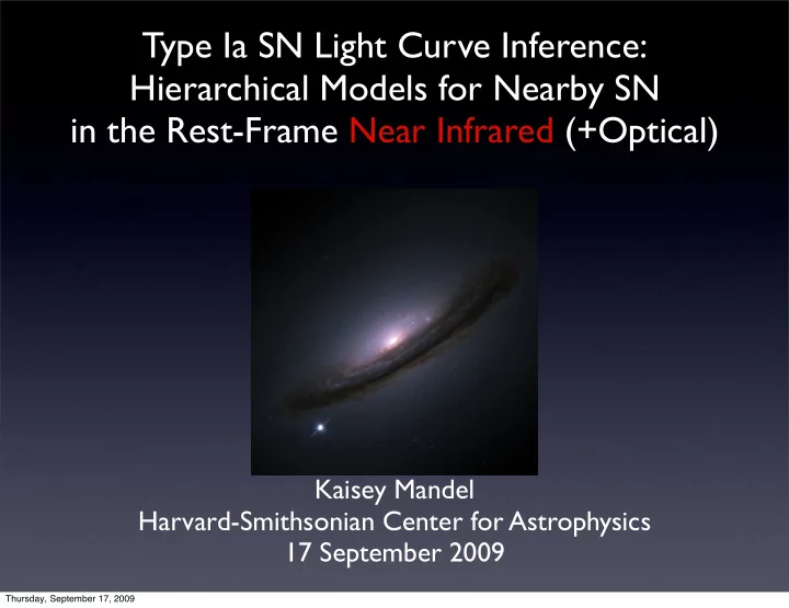
Type Ia SN Light Curve Inference: Hierarchical Models for Nearby SN - PowerPoint PPT Presentation

Type Ia SN Light Curve Inference: Hierarchical Models for Nearby SN in the Rest-Frame Near Infrared (+Optical) Kaisey Mandel Harvard-Smithsonian Center for Astrophysics 17 September 2009 Thursday, September 17, 2009

Outline • Statistical Inference with SN Ia Light curves • Hierarchical Framework for Constructing Probability Models for Observed Data • Describing Populations & Individuals • Statistical Computation with Hierarchical Models • BayeSN (MCMC/Gibbs Sampling) • Application to Nearby CfA NIR Data (PAIRITEL) 2 Thursday, September 17, 2009

For more details: Mandel, K. , W.M. Wood-Vasey, A.S. Friedman, R.P . Kirshner. Type Ia Supernova Light Curve Inference: Hierarchical Bayesian Analysis in the Near Infrared. 2009, ApJ, in press (October). preprint: arXiv:0908.0536 Collaborators: W. Michael Wood-Vasey (University of Pittsburgh), Andrew Friedman, Gautham Narayan, Malcolm Hicken, Pete Challis, Robert Kirshner CfA Supernova Group Thursday, September 17, 2009

Statistical Learning from SN Ia is a complex inference problem • Empirical statistical models are learned from the data • Several Sources of Randomness & Uncertainty • Photometric errors (Observational Noise) • “Intrinsic Variation” = Population Distribution of SN Ia • Variations in light curve shape over time, intrinsic color and luminosity vs λ : intrinsic correlation structure of SN Ia observeables • Random Peculiar Velocities in Hubble Flow • Host Galaxy Dust: extinction and reddening. • How to incorporate this all into a coherent statistical model? 4 Thursday, September 17, 2009

Advantages of Hierarchical Models • Coherently and simultaneously incorporate multiple sources of randomness & uncertainty: express complex probability models • Hierarchically Model (Physical) Populations and Individuals simultaneously: e.g. SN Ia and Dust • Can model both intrinsic variations/correlations in color/luminosity/ light curve shape and dust reddening and extinction for populations and individuals • Explore & Marginalize over posterior trade-offs/joint distributions • Get full probability distribution not just point estimates: • global, coherent quantification of uncertainties, • can compute complete marginalization over posterior uncertainties • Modularity: Can incorporate additional statistical structure to parts of the global model & condition on additional information (e.g. host galaxy type/environment, dust laws) Thursday, September 17, 2009

Directed Acyclic Graph for SN Ia Inference with Hierarchical Modeling • Intrinsic Randomness “Training” - Learn • Dust Extinction & Reddening about Populations • Peculiar Velocities • Measurement Error z 1 µ 1 Dust Av, Rv Pop #1 Generative Model AppLC D 1 AbsLC #1 Global Joint #1 Posterior µ N z N Av, Rv Probability AbsLC #N AppLC D N Density Pop #N Conditional on all AbsLC #N SN Data 6 Thursday, September 17, 2009

Directed Acyclic Graph for SN Ia Inference: Distance Prediction z s µ s A s V , R s V Dust AppLC s AbsLC s D s Pop s = 1 , . . . , N SN Training A p V , R p SN Ia Prediction µ p V AbsLC Pop AppLC p AbsLC p D p 7 Thursday, September 17, 2009

Statistical Computation with Hierarchical SN Ia Models: The BayeSN Algorithm • S trategy: Generate a 0.9 1 0.8 2 Markov Chain to sample 3 0.7 global parameter space A V Dust Extinction 0.6 (populations & all 0.5 individuals) using Gibbs 0.4 Sampling => seek a global 0.3 0.2 sol’n 0.1 • Chain explores/samples 0 0 1 2 3 10 10 10 10 MCMC Chain Sample trade-offs/degeneracies in Multiple chains globally global parameter space converge from random for populations and individuals initial values Thursday, September 17, 2009

Practical Application of Hierarchical Model: NIR SN Ia Why are NIR SN Ia interesting? • Host Galaxy Dust presents a major systematic uncertainty in supernova cosmology inference • Dust extinction has significantly reduced effect in NIR bands • NIR SN Ia are good standard candles (Elias et al. 1985, Meikle 2000, Krisciunas, et al. 2004+, Wood-Vasey, et al. 2008, Mandel et al. 2009). • Observe in NIR !: PAIRITEL / CfA 9 Thursday, September 17, 2009

NIR Observations from PAIRITEL Observe in NIR bands J ( λ =1.2 μ m) H ( λ =1.6 μ m) Ks ( λ =2.2 μ m) Credit: Andrew Friedman 10 Thursday, September 17, 2009

Nearby SN Ia in the NIR: The Training Data Credit: Michael Wood-Vasey, Andrew Friedman WV08 Data Set = PAIRITEL + Lit = 39 SN Ia in NIR Working on 40-60 more SNe (Andy Friedman) 11 Thursday, September 17, 2009

Light-curve shape variations in NIR 0 Normalized Magnitude 1 • Double-Peak light-curve 2 d / α = 1 ± 0.3 r / β = 1 ± 0.3 3 structure seen in JHK 0 Normalized Magnitude bands 1 • Difficult to capture with 2 α = 1 ± 0.3 β = 1 ± 0.3 3 one parameter 0 20 40 60 0 20 40 60 (T − T Bmax ) / (1+z) (T − T Bmax ) / (1+z) • J-band LC Model captures − 0.5 J (39 SNe Ia) 0 timescales and amplitudes 0.5 of late-time NIR light 1 J − J 0 1.5 curves (Mandel et al. 2 2009) 2.5 3 J − band FLIR Template Original Data 3.5 Transformed Data − 10 0 10 20 30 40 50 60 Time Since T Bmax Thursday, September 17, 2009

SN NIR Population Inference: Peak Absolute Magnitudes Marginal Distributions of SN Ia NIR Population characteristics • Marginal Estimate of K s J H Population Variance in 0.3 H-band (1.6 μ m) is µ (M H ) = − 18.00 0.25 σ (M H ) = 0.11 σ (M H ) = 0.11± 0.03 mag σ (M X ) 0.2 0.15 • SN Ia in NIR are excellent standard 0.1 µ (M J ) = − 18.26 µ (M Ks ) = − 18.24 candles! σ (M J ) = 0.17 σ (M Ks ) = 0.18 0.05 − 18.35 − 18.15 − 18.1 − 17.9 − 18.35 − 18.15 µ (M J ) µ (M H ) µ (M Ks ) Mandel et al. 2009 Thursday, September 17, 2009

Hubble Diagram with nearby NIR SN Ia Hubble Residuals of 36 h = 0.72 Hierarchical NIR σ pec = 150 km/s µ (resub) 34 SN Ia Model Fit 32 Bootstrap Cross- 39 JHK s distance moduli 30 Validation: 3 4 10 10 To Estimate effect of 0.5 finite sample size Residual 0 ~ 0.05 mag: Need larger sample − 0.5 Residual Err (cz > 2000 km/s) = 0.10 (Friedman, Wood-Vasey) 3 4 10 10 Velocity [CMB+Virgo] (km/s) Mandel et al. 2009 Thursday, September 17, 2009

Preview: Optical+NIR Hierarchical Inference PTEL+CfA3 Light-curves Marginal Posterior of Dust 0.08 6 0.07 SN2006ax H � 9 8 0.06 10 NIR Extinction A H J � 7 Apparent Magnitude 0.05 12 I � 4 0.04 14 R � 2 0.03 16 V (Preliminary) 0.02 18 0.01 20 SN2006ax (CfA3+PTEL) B + 2 0 22 0.1 0.2 0.3 0.4 0.5 0.6 0.7 � 10 0 10 20 30 40 50 60 � 1 Dust Law Slope R V T � T Bmax 6 8 0.25 H � 9 10 SN2005eq J � 7 0.2 NIR Extinction A H Apparent Magnitude 12 I � 4 14 0.15 R � 2 16 0.1 18 V 20 0.05 SN2005eq (CfA3+PTEL) B + 2 22 0 � 10 0 10 20 30 40 50 60 0.1 0.2 0.3 0.4 0.5 0.6 T � T Bmax � 1 Dust Law Slope R V Thursday, September 17, 2009

Summary • Hierarchical models are useful statistical constructions for incorporating multiple levels of randomness affecting SN Ia inference and modeling physical populations coherently • BayeSN: an efficient MCMC/Gibbs Sampler for computing hierarchical models conditional on SN data • NIR Light Curves give excellent distances less prone to dust extinction • Use Optical with NIR to estimate dust and make Type Ia SN better standard candles (work in progress!) • Rest-Frame NIR observations of SN Ia: consideration for JDEM 16 Thursday, September 17, 2009