Transient Lumped Parameter Analysis of Heat Pipe for a Space Nuclear - PDF document

Transactions of the Korean Nuclear Society Virtual Spring Meeting July 9-10, 2020 Transient Lumped Parameter Analysis of Heat Pipe for a Space Nuclear Reactor Nam-il Tak, * Sung Nam Lee Korea Atomic Energy Research Institute, 111, Daedeok-daero 989 Beon-gil, Yuseong-gu, Daejeon 34057, Korea *Corresponding author: takni@kaeri.re.kr 𝑞𝑓 ). In addition, ‘+’ is used for incoming heat flow to 1. Introduction 𝑈 node i whereas ‘ - ’ is used for outgoing heat flow from node i . Korea Atomic Energy Research Institute (KAERI) has been developing a design concept and key technologies for a space nuclear reactor [1,2]. The space nuclear reactor adopts a heat pipe to transfer the nuclear fission heat to an electricity generating device, e.g., stirring engine. The heat pipe is a capillary-driven and two-phase flow device. It is attractive in space since it is capable of transporting large amount of heat using passive and reliable manners with small sizes. This paper describes a lumped parameter numerical model which is able to simulate steady-state as well as transient operation of the heat pipe. Although the physical mechanisms related to transient heat pipe operation are numerous and complex, transient response of a heat pipe has been well studied and functional detailed models such as THROHPUT [3] and HPTAM Fig. 1. Thermal network of the present heat pipe model. [4] are already available. However, it is doubtful that such levels of details are necessary in engineering- approach simulation of a heat pipe (in particular, under a For the vapor temperatures (𝑈 𝑤𝑑 ) , quick thermal 𝑤𝑓 , 𝑈 conceptual design stage). equilibrium is assumed in this work. The main objective of the present work is to build a 𝑈 𝑥𝑓 − 𝑈 = 𝑈 𝑤𝑑 − 𝑈 = 𝑈 𝑤𝑓 − 𝑈 simple, reliable, and robust numerical model to design 𝑤𝑓 𝑥𝑑 𝑤𝑑 = 𝑅 𝑢𝑠𝑏𝑜𝑡 (2) 𝑆 2𝑥𝑓 + 𝑆 𝐹 𝑆 2𝑥𝑑 + 𝑆 𝐷 𝑆 𝑊 and analyze a heat pipe for practical engineering applications. where 𝑅 𝑢𝑠𝑏𝑜𝑡 = amount of heat transfer by vapor flow. Such an assumption can be justified by the fact that heat 2. Numerical Method capacity of vapor is much smaller than that of wick or pipe. For example, the volumetric heat capacity of A lumped parameter model was adopted in this work saturated sodium vapor is less than 0.02 % of stainless due to its simplicity as well as popularity in heat pipe steel 304 at 900 o C. applications. The lumped parameter model was adopted The analytical expressions of thermal resistances for by classical computer programs (e.g., HTPIPE [5] and pipe and wick are: ( 𝑠𝑓 ANL/HTP [6]) as well as recent researches (e.g., ln⁡ ) 𝑠𝑗 𝑆 𝑠𝑏𝑒𝑗𝑏𝑚 = Ferrandi et al.’s work [7]). 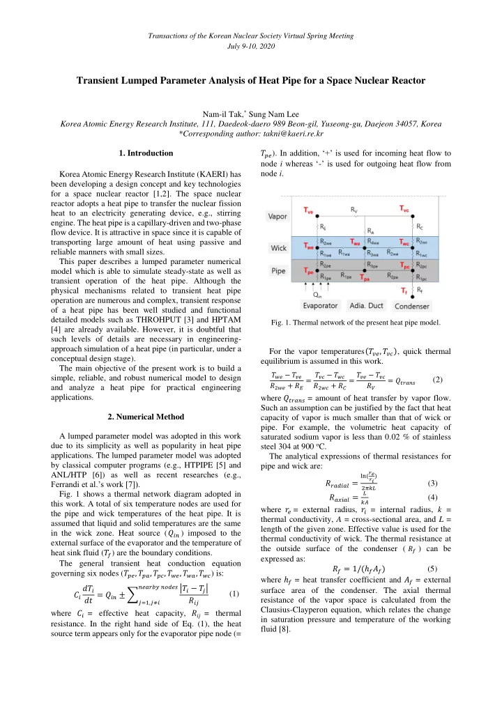(3) 2𝜌𝑙𝑀 𝑀 Fig. 1 shows a thermal network diagram adopted in 𝑆 𝑏𝑦𝑗𝑏𝑚 = (4) 𝑙𝐵 this work. A total of six temperature nodes are used for where 𝑠 𝑓 = external radius, 𝑠 𝑗 = internal radius, k = the pipe and wick temperatures of the heat pipe. It is thermal conductivity, A = cross-sectional area, and L = assumed that liquid and solid temperatures are the same length of the given zone. Effective value is used for the in the wick zone. Heat source ( 𝑅 𝑗𝑜 ) imposed to the thermal conductivity of wick. The thermal resistance at external surface of the evaporator and the temperature of the outside surface of the condenser ( 𝑆 𝑔 ) can be heat sink fluid ( 𝑈 𝑔 ) are the boundary conditions. expressed as: The general transient heat conduction equation 𝑆 𝑔 = 1/(ℎ 𝑔 𝐵 𝑔 ) (5) governing six nodes ( 𝑈 𝑞𝑓 , 𝑈 𝑞𝑏 , 𝑈 𝑞𝑑 , 𝑈 𝑥𝑓 , 𝑈 𝑥𝑏 , 𝑈 𝑥𝑑 ) is: where ℎ 𝑔 = heat transfer coefficient and 𝐵 𝑔 = external 𝑒𝑈 𝑜𝑓𝑏𝑠𝑐𝑧 𝑜𝑝𝑒𝑓𝑡 |𝑈 𝑗 − 𝑈 𝑘 | surface area of the condenser. The axial thermal 𝑗 (1) 𝐷 𝑗 𝑒𝑢 = 𝑅 𝑗𝑜 ± ∑ 𝑆 𝑗𝑘 resistance of the vapor space is calculated from the 𝑘=1,𝑘≠𝑗 Clausius-Clayperon equation, which relates the change where 𝐷 𝑗 = effective heat capacity, 𝑆 𝑗𝑘 = thermal in saturation pressure and temperature of the working resistance. In the right hand side of Eq. (1), the heat fluid [8]. source term appears only for the evaporator pipe node (=

Transactions of the Korean Nuclear Society Virtual Spring Meeting July 9-10, 2020 𝑈 𝑏𝑤𝑓 ⁡∆𝑄 𝑆 𝑊 = 𝜍 𝑏𝑤𝑓⁡ ℎ 𝑔𝑕 ⁡𝑅 𝑢𝑠𝑏𝑜𝑡 (6) where 𝑈 𝑏𝑤𝑓 = average temperature, ∆P = vapor pressure Table I: Heat Pipe Module Dimensions drop, 𝜍 𝑏𝑤𝑓 = average density, ℎ 𝑔𝑕 = latent heat of Item Value vaporization. The thermal resistance at the boiling and Heat pipe length (cm) 120 condensing surfaces are calculated using the model Evaporator length (cm) 43 presented by Dunn and Reay [9]. The model uses the Condenser length (cm) 77 Clausius-Clayperon relationship for saturated vapor and Heat pipe outside diameter (cm) 2.54 the fact that the evaporating or condensing mass Heat pipe inside diameter (cm) 2.21 transport is proportional to the heat transport. In case of Wick outside diameter (cm) 2.07 boiling at the evaporator, the thermal resistance at the Annular gap thickness (cm) 0.07 liquid-vapor interface is derived as: Wick inside diameter (cm) 1.74 𝑆 𝐹 = √2𝜌𝑆𝑈⁡𝑆𝑈 2 Wick thickness (cm) 0.17 𝑄⁡ℎ 𝑔𝑕2 𝐵 𝐹 (7) Effective pore radius (  m) 47 where R = gas constant of vapor, P = pressure, and 𝐵 𝐹 = surface area for evaporation. A similar expression for condensing (= 𝑆 𝐷 ) can be defined by replacing the There was no adiabatic zone in the heat pipe. The condenser of the heat pipe was exposed to ambient air surface area only. Since the thermal resistances 𝑆 𝑊 , 𝑆 𝐹 , 𝑆 𝐷 depend on the with room temperature and totally cooled by thermal radiation. The heat pipe was heated from room vapor temperature, iterative calculations are necessary to temperature. The heater power was increased to the heat obtain the vapor temperature. pipe module in 80 W increments at five minute intervals Eqs. (1) ~ (7) can be solved simultaneously by using a until 3 hours, kept constant during 0.5 hour, and standard numerical solver for combined ordinary decreased slowly during 1.5 hours. Fig. 3 shows the differential equations. applied heat input to the heat pipe. It was assumed that 3. Validation Results and Discussions the heat input was linearly applied. The reference [10] reported that the peak power was 660 W at the measured The feasibility of the present method was studied by peak surface temperature of the heat pipe (=900 K). using the Los Alamos National Laboratory (LANL) Using this information, the emissivity of the heat pipe experiment using a sodium heat pipe [10]. Stainless steel was estimated by the analytic expression of radiation sodium heat pipe modules were built and tested at LANL heat transfer in this work. for use in a thermo-hydraulic simulation of a space nuclear reactor. A cutaway drawing of the heat pipe module with its four cartridge heater is shown in Fig. 2. The major dimensions of the heat pipe are provide in Table I. The annular wick was fabricated from 304 L stainless steel screens. The wick consists of one support layer of 100-mesh screen, three capillary pumping layers of 400-mesh screen, and two liquid flow layers of 60- mesh screen. The test for the effective pore radius verified that the pore radius of the wick was less than 47 microns. Fig. 3. Applied heat input vs time. Fig. 4 compares the predicted and measured surface temperature of the heat pipe. A good agreement is shown in higher temperature region whereas some deviations exist in lower temperature region. It seems that the discrepancy in lower temperature region is mainly due to Fig. 2. Cutaway view of sodium heat pipe used for the LANL Eqs. (6) and (7), which are valid for small temperature experiment [10]. difference of vapor between the evaporator and the condenser. Improved models are necessary for accurate simulation of start-up behavior of the heat pipe. Fig. 5 shows the calculated heat removal by vapor and the operational limits of the heat pipe. During early stage of the experiment, the vapor heat transport is slightly