Lumped parameter model Lumped parameter models describe the - PDF document

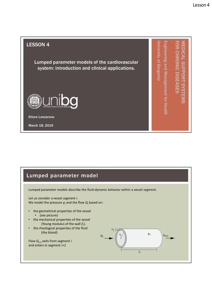
Lesson 4 University of Bergamo Engineering and Management for Health FOR CHRONIC DISEASES MEDICAL SUPPORT SYSTEMS LESSON 4 Lumped parameter models of the cardiovascular system: introduction and clinical applications. Ettore Lanzarone March 18, 2019 Lumped parameter model Lumped parameter models describe the fluid-dynamic behavior within a vessel segment. Let us consider a vessel segment i . We model the pressure p i and the flow Q i based on: • the geometrical properties of the vessel • (see picture) • the mechanical properties of the vessel (Young modulus of the wall E i ). • the rheological properties of the fluid (the blood) Flow Q i+1 exits from segment i and enters in segment i+1

Lesson 4 Lumped parameter model They are lumped because the concentrate the pressure and the flow in all points of the vessel into only two variables: pressure p i and the flow Q i . Blood rheology Blood is a suspension of particles ( erythrocytes, leukocytes and thrombocytes ) in aqueous solution ( the plasma ). In general it can not be considered a homogeneous fluid. It can be assumed homogeneous when it flows into vessels whose lumen is much greater than the size of the erythrocytes: up to small arteries with an internal diameter of 0.3 mm . In these cases, the blood is characterized simply by its density and its viscosity. When blood flows in smaller vessels, it is no longer correct to use a homogeneous fluid model, but it is still possible to define an apparent viscosity to avoid distinguishing the different components.

Lesson 4 Blood rheology Blood density is given by the average between the density of the plasma and that of the corpuscular part, weighed on the volume fraction of the two components. The fraction in volume of the corpuscular part is the Hematocrit Ht . Thus:        ρ ρ Ht ρ 1 Ht blood corpuscola r plasma - the density of the corpuscular part is equal to 1095 kg/m 3 - the density of plasma is equal to 1030 kg/m 3 The density is independent of temperature. Blood rheology When it is considered homogeneous, blood is treated as a Newtonian fluid (viscosity independent of motion conditions). The viscosity of plasma is given by the Lightfoot relationship:   μ 1 . 8 μ plasma water The viscosity of water in function of the temperature is given by the Poiseuille relation: μ  μ water 0     2 1 0 . 0337 T 0 . 00022 T T is the temperature expressed in Celsius [ o C ] μ 0 is the viscosity of water at o C , equal to 1.888 cP

Lesson 4 Blood rheology Finally, the viscosity of whole blood is given by the Bull relationship:       μ μ 1 2 . 5 Ht blood plasma Ht is once again the hematocrit Summing up, the viscosity of the whole blood is expressed in function of temperature and hematocrit as:      1 . 8 1 2 . 5 Ht  μ blood 1 . 808 cP     2 1 0 . 0337 T 0 . 00022 T Blood rheology In small-diameter vessels, the corpuscular fraction tends to occupy the central part of the vessel, with the red blood cells arranged perpendicular to the capillary axis, while the plasma is placed in the part closest to the wall. In this configuration, the plasma has a lubricating effect: the internal friction of the blood is reduced and the viscosity is therefore lower. By further reducing the diameter, the erythrocytes are forced to deform to advance; this increases energy losses and thus the viscosity.

Lesson 4 Blood rheology Progressively reducing the diameter, the viscosity first decreases and then tends to rise again: Fahareus-Lindqvist effect Blood rheology In this case, we can anyway define an “apparent” viscosity that defines the overall behavior in function of the vessel diameter.     C   Ht   2 2 1 1    D   D  100            μ μ 1 μ 1     apparent plasma 45   C D 1 , 1 D 1 , 1     45     1 1   100 with: D internal diameter in μm Ht hematocrit in percentage    1  1    0 , 075  D     C 0 , 8 e  1     11  12  11  12  1 10 D  1 10 D μ 0 , 645       Bull - 0 , 085 D - 0 , 06 D μ 6 e - 2 , 44 e 45 μ plasma μ Bull is the viscosity according to the Bull relationship

Lesson 4 Blood rheology Vessel model with electrical analogy The state variables are the average pressure p i and the flow Q i in the i -th segment. The parameters are: • Resistance R i : viscous hydraulic resistance which opposes the advancement of the blood. • Compliance C i : capacitive effect due to the elastic behavior of the walls. • Inertance L i : inertial effect linked to the motion of blood in the vessels. • Viscous resistance of the wall RV i : dissipative effect linked to the viscous behavior of the walls. All these parameters are calculated starting from the rheological properties of the blood ( density and viscosity ) and the geometrical and mechanical characteristics of the vessel ( internal radius, thickness of vessel walls, length and radial Young modulus of the walls ).

Lesson 4 Vessel model with electrical analogy The fluid dynamic equations are obtained starting from: • continuity equation (i.e., mass conservation )  capacitive effect deriving from the conservation of the mass • energy balance  resistive and inertial effects deriving from the energy balance The dissipative element relative to the viscosity of the wall is then added. Vessel model with electrical analogy dM    The conservation of the mass can be written as:  m m 1 2 dt M is the mass contained in the segment 𝑛 ̇ is the mass flow rate (subscript 1 for mass entering the vessel segment and subscript 2 for mass leaving the vessel segment). Considering a constant density ρ and denoting by V the volume and by Q the volumetric flow, the expression becomes: dV     ρ ρ Q ρ Q 1 2 dt dV   Q Q 1 2 dt

Lesson 4 Vessel model with electrical analogy dV C  We now include the definition of Compliance: dp Thus, the first equation for the vessel motion is: dp   C Q Q 1 2 dt Vessel model with electrical analogy The second equation is obtained with the energy balance, under the hypothesis that the incoming mass flow equals the outgoing one. The energy balance is:     2 2 dE p p v v           m  1 2 m  β 1 β 2 m  ΔH     1 2 dt ρ ρ 2 2     where: • E is the energy; • v is the velocity; • ΔH the energy dissipation per unit of time due to blood viscosity; • β is a multiplicative coefficient linked to the motion regime. Subscript 1 is incoming quantities and subscript 2 for outgoing quantities. The difference in altitude between input and the output is neglected.

Lesson 4 Vessel model with electrical analogy Energy is only kinetic energy (neglecting thermal effects): 2 2 v v    2  E M ρ πr l 2 2 Its derivative is (with constant radius): dE dv dv   2     ρ πr l v m  l dt dt dt Vessel model with electrical analogy Thus, the energy balance is:     2 2 dv p p v v            m  l m  1 2 m  β 1 β 2 m  ΔH     1 2 dt ρ ρ 2 2     The terms related to the velocity are equal and are simplified (same input and output flow and same cross sections). dv Thus:      p p ρ l ρ ΔH 1 2 dt  ρ l dQ      p p ρ ΔH 1 2  2 π r dt

Lesson 4 Vessel model with electrical analogy  ρ l dQ      p p ρ ΔH 1 2  2 π r dt is rewritten as: dQ     p p L R Q 1 2 dt Vessel model with electrical analogy The two equations that describe the fluid dynamics are: dp   C Q Q 1 2 dt Dynamical system described by two ODEs of dQ the first order for the two     p p L R Q state variables p and Q 1 2 dt Now: - How to determine the parameters R, L and C based on mechanical and geometrical properties. - How to describe in terms of an electrical circuit. - How to attach the viscosity of the vessel walls.

Lesson 4 Vessel model with electrical analogy COMPLIANCE C We assume a thin-walled vessel. Under this assumption, the compliance C is determined with the Laplace law:   T p r ( T is the circumferential tension in the wall) By differentiating this law we have:     dT p dr r dp Vessel model with electrical analogy dT is expressed as a function of the infinitesimal circumferential deformation dr : dr  dε r dσ dT   dε  E s E where E is the Young modulus of the vessel walls. Thus: dr   dT s E r