10/16/19 Parameters and Parameter Tuning Genetic Algorithms - - PDF document

10/16/19 1

Genetic Algorithms

Parameters and Parameter Tuning Parameters and Parameter Tuning

• History
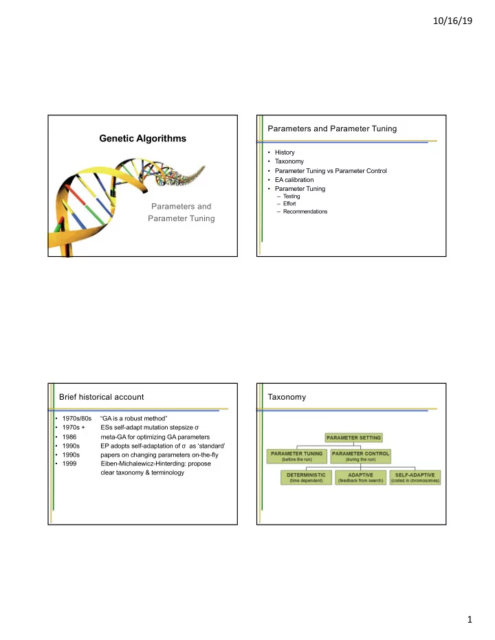
• Taxonomy
• Parameter Tuning vs Parameter Control
• EA calibration
• Parameter Tuning

– Testing – Effort – Recommendations

Brief historical account

• 1970s/80s “GA is a robust method”
• 1970s + ESs self-adapt mutation stepsize σ
• 1986 meta-GA for optimizing GA parameters
• 1990s EP adopts self-adaptation of σ as ‘standard’
• 1990s papers on changing parameters on-the-fly
• 1999 Eiben-Michalewicz-Hinterding: propose

clear taxonomy & terminology

Taxonomy

10/16/19 2

Parameter tuning

Parameter tuning: testing and comparing different values before the “real” run – part of development Problems:

– user “mistakes” in settings can be sources of errors or sub-

• ptimal performance

– takes significant time – parameters interact: exhaustive search is not practical (or even possible, in some cases) – good values may become bad during the run (at different stages

• f evolutionary development in the population)

Parameter control

Parameter control: setting values on-line, during the actual run, e.g.

— predetermined time-varying schedule p = p(t) — using (heuristic) feedback from the search process — encoding parameters in chromosomes and rely on natural selection

Problems:

— finding optimal p is hard, finding optimal p(t) is harder — still user-defined feedback mechanism, how to “optimize”? — when would natural selection work for algorithm parameters?

Notes on parameter control

• Parameter control offers the possibility to use appropriate values in

various stages of the search

• Adaptive and self-adaptive control can “liberate” users from tuning à

reduces need for EA expertise for a new application

• Assumption: control heuristic is less parameter-sensitive than the EA

BUT

• State-of-the-art is a mess: literature is a potpourri, no generic

knowledge, no principled approaches to developing control heuristics (deterministic or adaptive), no solid testing methodology

Historical account (cont’d)

Last 20 years:

• More & more work on parameter control

– Traditional parameters: mutation and xover – Non-traditional parameters: selection and population size – All parameters è “parameterless” EAs (what to call these?) – Some theoretical results (e.g. Carola Doerr)

• Not much work on parameter tuning, i.e.,

– Nobody reports on tuning efforts behind their published EAs (common refrain: “values were determined empirically”) – A handful of papers on tuning methods / algorithms

10/16/19 3

Parameter – performance landscape

— All parameters together span a (search) space — One point – one EA instance — Height of point = performance of EA instance on a given problem — Parameter-performance landscape or utility landscape for each { EA + problem instance + performance measure } — This landscape is likely to be complex e.g., multimodal — If there is some structure in the utility landscape, then perhaps we can do better than random or exhaustive search

The Tuning Problem

• Parameter values determine the success and efficiency
• f a genetic algorithm
• Parameter tuning is a method in which parameter values

determined before a run and remain fixed during

• Common approaches:

– Convention, e.g. mutation rate should be low; xover rate = 0.9 – Ad hoc choices, e.g. let’s use population size of 100 – Limited experimentation, e.g. let’s try a few values

The Tuning Problem Problems

• Problems with convention and ad hoc choices are
• bvious

– Were choices ever justified? – Do they apply in new problem domains?

• Problems with experimentation

– Parameters interact – cannot be optimized one-by-one – Time consuming: 4 parameters with 5 values each yields 625 parameter combinations. 100 runs each = 62500 runs just for tuning – to be fair, any tuning method will be time consuming – Best parameter values may not be in test set

The Tuning Problem Goal

• Think of design of a GA as a separate search problem
• Then a tuning method is a search algorithm
• Such a tuning method can be used to:

– Optimize a GA by finding parameters that optimize its performance – Analyze a GA by studying how performance depends on parameter values and the problems to which it is applied

• So tuning problem solutions depend on problems to be

solved, GA used, and utility function that defines how GA quality is measured

10/16/19 4

The Tuning Problem Terminology

Problem Solving Algorithm Design METHOD EA Tuner SEARCH SPACE Solution vectors Parameter vectors QUALITY Fitness Utility ASSESSMENT Evaluation Test

— Fitness ≈ objective function value — Utility = ?

— Mean Best Fitness — Average number of Evaluations to Solution — Success Rate — Robustness, … — Combination of some of these

Defining Algorithm Quality

• GA quality generally measured by a combination of

solution quality and algorithm efficiency

• Solution quality – reflected in fitness values
• Algorithm efficiency

– Number of fitness evaluations – CPU time – Clock-on-the-wall time

Defining Algorithm Quality

• Three generally used combinations of solution quality

and computing time for single run of algorithm

– Fix computing time and measure solution quality

• Given maximum runtime, quality is best fitness at

termination – Fix solution quality and measure computing time required

• Given a minimum fitness requirement, performance is the

runtime needed to achieve it – Fix both and measure success

• Given maximum runtime and minimum fitness requirement,

run is successful if it achieves fitness requirement within runtime limit

Tuning Methods Off-line vs. on-line calibration / design

Design / calibration method — Off-line à parameter tuning — On-line à parameter control — Advantages of tuning

— Easier — Most immediate need of users — Control strategies have parameters too à need tuning themselves — Knowledge about tuning (utility landscapes) can help the design of good control strategies — There are indications that good tuning works better than control

10/16/19 5

Tuning Method Tuning by generate-and-test

• Generate-and-test is a common search strategy
• Since EA tuning is a search problem itself…
• Straightforward approach:

Generate parameter vectors Test parameter vectors

Terminate All tuning methods are a form of generate-and-test

Generate-and-test Testing parameter vectors

— Run EA with these parameters on the given problem or problems — Record EA performance in that run e.g., by

— Solution quality = best fitness at termination — Speed ≈ time used to find required solution quality

— EAs are stochastic à repetitions are needed for reliable evaluation à we get statistics, e.g.,

— Average performance by solution quality, speed (MBF, AES) — Success rate = % runs ending with success — Robustness = variance in those averages over different problems

— Question: how many repetitions of the test (yet another “parameter”)

Definitions

• Because GAs are stochastic, single runs don’t tell us

much about the quality of an algorithm

• Aggregate measures over multiple runs:

– MBF: Mean Best Fitness – AES: Average evaluations to solution – SR: Success rate

Generate-and-Test Numeric parameters

• E.g., population size, xover rate, tournament size, …
• Domain is subset of R, Z, N (finite or infinite)
• Values are well ordered à searchable

Parameter value EA performance Parameter value EA performance

Relevant parameter Irrelevant parameter

10/16/19 6

Generate-and-test Symbolic parameters

• E.g., xover_operator, elitism, selection_method
• Finite domain, e.g., {1-point, uniform, averaging}, {Y, N}
• Values not well ordered à non-searchable, must be

sampled

• A value of a symbolic parameter can introduce a numeric

parameter, e.g., – Selection = tournament à tournament size – Populations_type = overlapping à generation gap – Elitism = on à number of best members to keep

What is an EA?

ALG-1 ALG-2 ALG-3 ALG-4 SYMBOLIC PARAMETERS Representation Bit-string Bit-string Real-valued Real-valued Overlapping pops N Y Y Y Survivor selection ̶ Tournament Replace worst Replace worst Parent selection Roulette wheel Uniformdeterm Tournament Tournament Mutation Bit-flip Bit-flip N(0,σ) N(0,σ) Recombination Uniform xover Uniform xover Discrete recomb Discrete recomb NUMERIC PARAMETERS Generation gap ̶ 0.5 0.9 0.9 Population size 100 500 100 300 Tournament size ̶ 2 3 30 Mutation rate 0.01 0.1 ̶ ̶ Mutation stepsize ̶ ̶ 0.01 0.05 Crossover rate 0.8 0.7 1 0.8

What is an EA?

Make a principal distinction between EAs and EA instances and place the border between them by: — Option 1 — There is only one EA, the generic EA scheme — Previous table contains 1 EA and 4 EA-instances — Option 2 — An EA = particular configuration of the symbolic parameters — Previous table contains 3 EAs, with 2 instances for one of them — Option 3 — An EA = particular configuration of parameters — Notions of EA and EA-instance coincide — Previous table contains 4 EAs / 4 EA-instances

Tuning effort

• Total amount of computational work is determined by

– A = number of vectors tested – B = number of tests per vector – C = number of fitness evaluations per test

10/16/19 7

Recommendations

• DO TUNE your evolutionary algorithm
• Think of the magic constants
• Decide: speed or solution quality?
• Decide: specialist or generalist EA?
• Measure and report tuning effort

Example study: ‘Best parameters’

• Setup:

– Problem: Sphere Function (see next slide) – EA: defined by Tournament Parent Selection, Random Uniform Survivor Selection, Uniform Crossover, BitFlip Mutation – Tuner: REVAC spending X units of tuning effort, tuning for speed

• Results: the best EA had the following parameter values
• Population Size: 6
• Tournament Size: 4
• Conclusions: for this problem we need a high (parent)

selection pressure.

Sphere Function (in 3 dimensions) Example study: ‘Good parameters’

• Setup: same as before
• Results: The 25 best parameters vectors have their values

within the following ranges

• Mutation Rate:

[0.01, 0.011]

• Crossover Rate: [0.2, 1.0]
• Conclusions: for this problem the mutation rate is much

more relevant than the crossover rate.

10/16/19 8

Example study: ‘interactions’

• Setup: same as before
• Results: plotting the pop.

size and generation gap of the best parameter vectors shows the following

• Conclusions: for this problem the best results are obtained

when (almost) the complete population is replaced every generation.

Generation Gap Population size

Control flow of EA calibration / design

De Design layer Ap Application layer Al Algorithm layer

• ptimizes
• ptimizes

One-max GA Meta-GA Symbolic regression GP User

Information flow of EA calibration / design

De Design layer Ap Application layer Al Algorithm layer Algorithm quality Solution quality

10/16/19 9

Lower level of EA calibration / design

Searches

Decision variables Problem parameters Candidate solutions

EA EA

Space of solution vectors

Evaluates Ap Application

Th The whole fi field o

• f E

f EC is is about this is

Upper level of EA calibration / design

De Design method Searches

Design variables, Algorithm parameters, Strategy parameters

Space of parameter vectors Evaluates EA EA

Optimize A = optimally use A

Applicable only to numeric parameters Number of tested vectors not fixed, A is the maximum (stop cond.) Population-based search:

– Initialize with N << A vectors and – Iterate: generating, testing, selecting p.v.’s

— Meta-EA (Greffenstette ‘86)

— Generate: usual crossover and mutation of p.v.’s

— SPO (Bartz-Beielstein et al. ‘05)

— Generate: uniform random sampling!!! of p.v.’s

— REVAC (Nannen & Eiben ’06)

— Generate: usual crossover and distribution-based mutation of p.v.’s

REVAC illustration

Time or fitness level

10/16/19 10

Optimize B = reduce B

Applicable to symbolic and numeric parameters Number of tested vectors (A) fixed at initialization Set of tested vectors can be created by — regular method à grid search — random method à random sampling — exhaustive method à enumeration Complete testing (single stage) vs. selective testing (multi-stage) — Complete testing: nr. of tests per vector = B (thus, not optimizing) — Selective testing: nr. of tests per vector varies, ≤ B — Idea:

— Execute tests in a breadth-first fashion (stages), all vectors X < B times — Stop testing vectors with statistically significant poorer utility

— Well-known methods

— ANOVA (Scheffer ‘89) — Racing (Maron & Moore ’97)

Optimize A & B

Existing work: — Meta-EA with racing (Yuan & Gallagher ‘04) New trick: sharpening (Smit & Eiben 2009) — Idea: test vectors X < B times and increase X over time during the run of a population-based tuner Newest method: — REVAC with racing & sharpening = REVAC++

Which tuning method?

— Differences between tuning algorithms

— Maximum utility reached — Computational costs — Number of their own parameters – overhead costs — Insights offered about EA parameters (probability distribution, interactions, relevance, explicit model…)

— Similarities between tuning algorithms

— Nobody is using them — Can find good parameter vectors

— Solid comparison is missing – ongoing

Tuning “world champion” EAs

G-CMA-ES SaDE Tuned by Avg St dev CEC Δ Avg St dev CEC Δ G-CMA-ES 0.77 0.2 20 % 0.73 0.25 49 % REVAC++ 0.85 0.24 12 % 0.67 0.22 53 % SPOT 0.76 0.19 22 % 0.73 0.20 49 % CEC-2005 0.97 0.32

• 1.43

0.25

• Main conclusion: if only they had asked us ….

Ranking at CEC 2005

• 1. CMA-ES
• 2. SaDE

Ranking after tuning

• 1. SaDE
• 2. CMA-ES

10/16/19 11

Tuning vs. not tuning

Performance EA 1 EA 2 Performance EA 1 EA 2 EA as is (accidental parameters) EA as it can be (“optimal” parameters)