Texture Mapping Motivation: Add interesting and/or realistic detail - PDF document

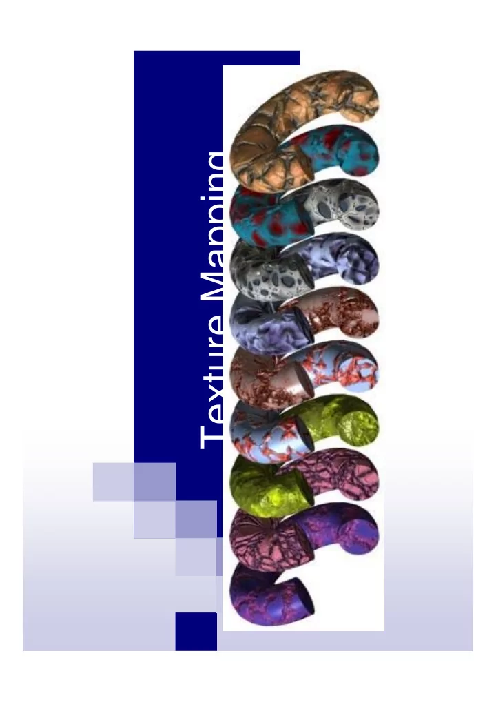
Texture Mapping

 Motivation: Add interesting and/or realistic detail to surfaces of objects.  Problem: Fine geometric detail is difficult to model and expensive to render.  Idea: Modify various shading parameters of the surface by mapping a function (such as a 2D image) onto the surface.

Textures and Shading 4 http://www.3drender.com/jbirn/hippo/hairyhipponose.html

Texture Mapping – Simple Example

Simple parametrization

Mapping is not unique

Bump Mapping

Bump Mapping

Surface Parametrization Most slides courtesy of Pierre Alliez, Craig Gotsman, and Noam Aigerman

Triangle mesh  Discrete surface representation  Piecewise linear surface (made of triangles) 13

Triangle mesh  Geometry:  Vertex coordinates (x 1 , y 1 , z 1 ) (x 2 , y 2 , z 2 ) . . . (x n , y n , z n )  Connectivity (the graph)  List of triangles (i 1 , j 1 , k 1 ) (i 2 , j 2 , k 2 ) . . . (i m , j m , k m ) 14

What is a parameterization? S  R 3 - given surface D  R 2 - parameter domain s : D  S 1-1 and onto   ( , ) x u v      ( , ) ( , ) s u v y u v    ( , )  z u v 15

16 Example – flattening the earth

Mesh Parameterization

18 World Atlas

Parameterizations are atlases

20 World Atlas

21 World Atlas

22 World Atlas

23 The true size of Africa

24 Another view of the same idea

There are many possible maps Is one of them “correct”?

Can’t flatten without distorting

Another example: Parameters:  , h D = [0,  ]  [ – 1,1] x (  , h ) = cos (  ) y (  , h ) = h h z (  , h ) = sin (  ) 1   -1 27

28 Triangular Mesh

29 Triangular Mesh

Mesh Parameterization  Uniquely defined by mapping mesh vertices to the parameter domain: U : {v 1 , …, v n }  D  R 2 U (v i ) = ( u i , v i )  No two edges cross in the plane (in D ) Mesh parameterization  mesh embedding 30

Mesh parameterization Parameterization s Embedding U Parameter domain Mesh surface D  R 2 S  R 3 s = U -1 31

2D parameterization 3D space ( x,y,z ) 2D parameter domain ( u,v ) boundary boundary 32

33 Application - Texture mapping

Requirements  Bijective (1-1 and onto): No triangles fold over.  Minimal “distortion”  Preserve 3D angles  Preserve 3D distances  Preserve 3D areas  No “stretch” 34

Distortion minimization Texture map Kent et al ‘92 Floater 97 Sander et al ‘01 35

36 More texture mapping

Resampling problems Cat mesh Distorting Resampling embedding on regular grid 37

Remeshing

39 Remeshing examples

40 Remeshing

41 Remeshing

42 More remeshing examples

Conformal parametrization Tutte Shape-preserving Conformal Texture map 43

44 Non-simple domains

45 Cutting

Parameterization of closed genus-0 triangle meshes Spherical Non-Constrained Planar 46

47 Introducing seams (cuts)

48 Partition

50 Introducing seams (cuts)

51 Introducing seams (cuts)

52 Bad parameterization

53 Better…(free boundary)

Partition – problems  Discontinuity of parameterization  Visible artifacts in texture mapping  Require special treatment  Vertices along seams have several (u,v) coordinates  Problems in mip-mapping Make seams short and hide them 54

Summary “Good” parameterization = non-distorting   Angles and area preservation  Continuous param. of complex surfaces cannot avoid distortion. “Good” partition/cut:   Large patches, minimize seam length  Align seams with features (=hide them) 55

Mesh parameterization s and U are piecewise-linear Linear inside each mesh triangle s U In 2D In 3D A mapping between two triangles is a unique affine mapping 56

Barycentric coordinates C P A B     , , , , , , P B C P C A P A B    P A B C , , , , , , A B C A B C A B C    , , denotes the (signed) area of the triangle 57

Mapping triangle to triangle s p 3 q 3 p 1 q 1 q 2 p 2 , , , , , , p p p p p p p p p    2 3 3 1 1 2 ( ) s p q q q 1 2 3 , , , , , , p p p p p p p p p 1 2 3 1 2 3 1 2 3 58

Some techniques

Convex mapping (Tutte, Floater)  Works for meshes equivalent to a disk  First, we map the boundary to a convex polygon  Then we find the inner vertices positions v 1 , v 2 , …, v n – inner vertices; v n , v n+1 , …, v N – boundary vertices 60

Inner vertices  We constrain each inner vertex to be a weighted average of its neighbors: j      1 , 2 , , v v , i n , i i j j  i,j  ( ) j N i i  0 , are not neighbors i j      , i j  0 ( , ) ( neighbours ) i j E    1 , i j  ( ) j N i 61

Linear system of equations       1 , 2 , , v v 0, i n , i i j j  ( ) j N i         1 , 2 , , v v v , i n , , i i j j i k k    ( ) \ ( ) j N i B k N i B            1 v       1 , 1 , j j 1 1 1 d 1        1 v 2 2        1                 4 , j       1    1     v   , n j n n 5 62

Shape preserving weights  1 v 3D p 1 2D p 5 v 1 v 4 p 2 v 5 p p 4 v 3 v 2 p 3 To compute  1 , …,  5 , a local embedding of the patch is found : 1) || p i – p || = || x i – x || 2) angle ( p i , p , p i+1 ) = (2  /   i ) angle ( v i , v , v i+1 ) p =   i p i  use these  as edge weights .  i > 0   i ,   i = 1 63

Linear system of equations  A unique solution always exists  Important: the solution is legal (bijective)  The system is sparse, thus fast numerical solution is possible  Numerical problems (because the vertices in the middle might get very dense…) 64

2D parameterization 3D space ( x,y,z ) 2D parameter domain ( u,v ) boundary boundary 65

Harmonic mapping  Another way to find inner vertices  Strives to preserve angles (conformal)  We treat the mesh as a system of springs.  Define spring energy: 1  2   E k v v , harm i j i j 2  ( , ) i j E where v i are the flat position (remember that the boundary vertices v n , v n+1 , …, v N are constrained). 66

Energy minimization – least squares  We want to find such flat positions that the energy is as small as possible.  Solve the linear least squares problem!  ( , ) v x y i i i 1  2      ( , , , , , ) E x x y y k v v 1 1 , harm n n i j i j 2  ( , ) i j E   . 1      2 2 ( ) ( ) k x x y y , i j i j i j 2  ( , ) i j E E harm is function of 2n variables 67

Energy minimization – least squares  To find minimum:  E harm = 0  1     2 ( ) 0 E k x x  harm i , j i j 2 x  ( ) j N i i  1     2 ( ) 0 E k y y  , harm i j i j 2 y  ( ) j N i i  Again, x n+1 ,…., x N and y n+1 , …, y N are constrained. 68

Energy minimization – least squares  To find minimum:  E harm = 0      ( ) 0 , 1 , 2 , , k x x i n i , j i j  ( ) j N i      ( ) 0 , 1 , 2 , , k y y i n , i j i j  ( ) j N i  Again, x n+1 ,…., x N and y n+1 , …, y N are constrained. 69

The spring constants k i,j  The weights k i,j are chosen to minimize angles distortion:  Look at the edge ( i, j ) in the 3D mesh  Set the weight k i,j = cot  + cot  i   3D j 70

Discussion  The results of harmonic mapping are better than those of convex mapping (local area and angles preservation).  But: the mapping is not always legal (the weights can be negative for badly-shaped triangles…)  Both mappings have the problem of fixed boundary – it constrains the minimization and causes distortion.  There are more advanced methods that do not require boundary conditions. 71

Convex weights for inner vertices      s.t. 1 and 0 v w v w w i ij j ij ij   ( , ) ( ) ( , ) ( ) i j N i i j N i  If the weights are convex, the solution is always valid (no self- intersections) [Floater 97]  The cotangent weight in Harmonic Mapping can be negative  sometimes there are triangle flips  In [Floater 2003] new convex weights are proposed that approximate harmonic mapping 72