[PPT] - Sol vi ng the LH C Confinement Showers h Amplitudes | M (0) H

SLIDE 1

P e t e r S k a n d s ( C E R N T H )

Sol vi ng the LH C

D I S C O V E R Y S e m i n a r, S e p 2 7 2 0 1 2 , N B I , C o p e n h a g e n

h |M (0)

H |2

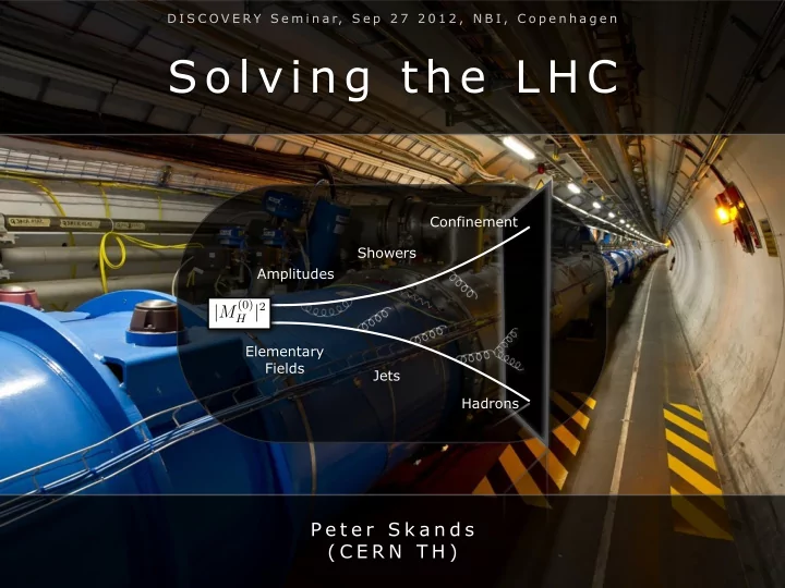
Amplitudes Showers Confinement Elementary Fields Jets Hadrons

SLIDE 2

P. S k a n d s

July 4th 2012: “Higgs- like” stuff at CERN

2

Why?

Precision = Clarity, in our vision of the Terascale

Searching towards lower cross sections, the game gets harder + Intense scrutiny (after discovery) requires high precision

Theory task: invest in precision This talk: a new formalism for highly accurate collider- physics predictions, and future perspectives

+ huge amount of other physics studies:

# of journal papers: 144 ATLAS, 116 CMS, 51 LHCb, 27 ALICE Some of these are already, or will ultimately be, theory limited

SLIDE 3

P. S k a n d s

How?

Fixed Order Perturbation Theory:

Problem: limited orders

Parton Showers:

Problem: limited precision

“Matching”: Best of both Worlds?

Problem: stitched together, slow

Markovian Perturbation Theory

→ Infinite orders, high precision, fast

3

SLIDE 4

P. S k a n d s

Accelerated Charges

Associated field (fluctuations) continues

Radiation Radiation

4

The harder they get kicked, the harder the fluctations that continue to become strahlung

Bremsstrahlung

SLIDE 5

P. S k a n d s

Bremsstrahlung

5

Most bremsstrahlung is emitted by particles that are almost on shell Divergent propagators → Bad fixed-order convergence

(would need very high orders to get reliable answer)

+ Would be infinitely slow to carry out separate phase- space integrations for N, N+1, N+2, etc …

SLIDE 6

P. S k a n d s

Jets = Fractals

6

Gauge amplitudes factorize in singular limits (→ universal

“conformal” or “fractal” structure)

i j k a b

Partons ab → collinear:

|MF +1(. . . , a, b, . . . )|2 a||b → g2

sC

P(z) 2(pa · pb)|MF (. . . , a + b, . . . )|2

P(z) = Altarelli-Parisi splitting kernels, with z = Ea/(Ea+Eb)

∝ 1 2(pa · pb)

+ scaling violation: gs2 → 4παs(Q2) Gluon j → soft:

|MF +1(. . . , i, j, k. . . )|2 jg→0 → g2

sC

(pi · pk) (pi · pj)(pj · pk)|MF (. . . , i, k, . . . )|2

Coherence → Parton j really emitted by (i,k) “antenna”

PS, Introduction to QCD, TASI 2012, arXiv:1207.2389

Can apply this many times → nested factorizations

Most bremsstrahlung is driven by Divergent propagators → simple structure

SLIDE 7

P. S k a n d s

Divide and Conquer

Factorization → Split the problem into many (nested) pieces

7

Pevent = Phard ⊗ Pdec ⊗ PISR ⊗ PFSR ⊗ PMPI ⊗ PHad ⊗ . . .

Hard Process & Decays:

Use (N)LO matrix elements → Sets “hard” resolution scale for process: QMAX

ISR & FSR (Initial & Final-State Radiation):

Altarelli-Parisi equations → differential evolution, dP/dQ2, as function of resolution scale; run from QMAX to ~ 1 GeV (More later)

MPI (Multi-Parton Interactions)

Additional (soft) parton-parton interactions: LO matrix elements → Additional (soft) “Underlying-Event” activity (Not the topic for today)

Hadronization

Non-perturbative model of color-singlet parton systems → hadrons

+ Quantum mechanics → Probabilities → Random Numbers

SLIDE 8

P. S k a n d s

Realized by Event evolution in Q = fractal scale (virtuality, pT, formation time, …)

Resolution scale t = ln(Q2) Probability to remain “unbranched” from t0 to t → The “Sudakov Factor” = Approximation to Real Emissions = Approximation to Loop Corrections

NF (t) NF (t0) = ∆F (t0, t) = exp ✓ − Z dσF +1 dσF ◆

dNF (t) dt = −dσF +1 dσF NF (t)

8

Last Ingredient: Loops

2Re[M(0)

F M(1)∗ F

] ⊃ −g2

s NC

M(0)

F

2 Z dsij dsjk

16⇡2sijk ✓ 2sik sijsjk + less singular terms ◆ that cancels the divergence coming from equation (52) itself. Further, since this is universally

=

→ Virtual (loop) correction:

Loop = - Int(Tree) + F

Neglect F → Leading-Logarithmic (LL) Approximation

Kinoshita-Lee-Nauenberg:

PS, Introduction to QCD, TASI 2012, arXiv:1207.2389

Unitarity (KLN): Singular structure at loop level must be equal and opposite to tree level

SLIDE 9

P. S k a n d s

Bootstrapped Perturbation Theory

9

→ All Orders (resummed)

Born + Shower

Unitarity Universality (scaling) Jet-within-a-jet-within-a-jet-...

X(2) X+1(2) … X(1) X+1(1) X+2(1) X+3(1) … Born X+1(0) X+2(0) X+3(0) … L

p

s L e g s

Exponentiation

But ≠ full QCD! Only LL Approximation.

SLIDE 10

P. S k a n d s

→ Jack of All Orders, Master of None?

Good Algorithm(s) → Dominant all-orders structures But what about all these unphysical choices?

Renormalization Scales (for each power of αs) The choice of shower evolution “time” ~ Factorization Scale(s) The radiation/antenna/splitting functions (finite terms arbitrary) The phase space map (“recoils”, dΦn+1/dΦn ) The infrared cutoff contour (hadronization cutoff)

10

1. Systematic

Variations

→ Comprehensive Theory Uncertainty Estimates

Nature does not depend on them → vary to estimate uncertainties Problem: existing approaches vary only one or two of these choices

2. Higher-Order Corrections

→ Systematic Reduction of

Uncertainties

SLIDE 11

P. S k a n d s

1 1 i j k I i j k I m+1 m+1 K K

VINCIA

11

Giele, Kosower, Skands, PRD 78 (2008) 014026, PRD 84 (2011) 054003 Gehrmann-de Ridder, Ritzmann, Skands, PRD 85 (2012) 014013

Virtual Numerical Collider with Interleaved Antennae Written as a Plug-in to PYTHIA 8 C++ (~20,000 lines)

Based on antenna factorization

of Amplitudes (exact in both soft and collinear limits)
of Phase Space (LIPS : 2 on-shell → 3 on-shell partons, with (E,p) cons)

Resolution Time

Infinite family of continuously deformable QE Special cases: transverse momentum, invariant mass, energy + Improvements for hard 2→4: “smooth ordering”

Radiation functions

Written as Laurent-series with arbitrary coefficients, anti Special cases for non-singular terms: Gehrmann-Glover, MIN, MAX + Massive antenna functions for massive fermions (c,b,t)

Kinematics maps

Formalism derived for infinitely deformable κ3→2 Special cases: ARIADNE, Kosower, + massive generalizations

0.2 0.2 0.4 0.4 0.6 0.6 0.8 0.8 0.0 0.2 0.4 0.6 0.8 1.0 0.0 0.2 0.4 0.6 0.8 1.0 yij yjk ⌦ ↵ 0.2 0.4 0.6 0.8 0.0 0.2 0.4 0.6 0.8 1.0 0.0 0.2 0.4 0.6 0.8 1.0 yij yjk (c) 2 ∗√ 0.2 0.4 0.6 0.8 0.0 0.2 0.4 0.6 0.8 1.0 0.0 0.2 0.4 0.6 0.8 1.0 yij yjk

pT mD Eg vincia.hepforge.org

SLIDE 12

P. S k a n d s

Changing Paradigm

12

Ask: Is it possible to use the all-orders structure that the shower so nicely generates for us, as a substrate, a stratification, on top of which fixed-order amplitudes could be interpreted as corrections, which would be finite everywhere? Answer: Used to be no. (Though first order worked out in the eighties (Sjöstrand), expansions rapidly became too complicated) For multileg amplitudes, people then resorted to slicing up phase space (fixed-order amplitude goes here, shower goes there), generated many different cookbook recipes and much bookkeeping

SLIDE 13

P. S k a n d s

Idea:

Start from quasi-conformal all-orders structure (approximate) Impose exact higher orders as finite corrections Truncate at fixed scale (rather than fixed order) Bonus: low-scale partonic events → can be hadronized

Problems:

Traditional parton showers are history-dependent (non-Markovian) → Number of generated terms grows like 2N N! + Highly complicated expansions

Solution: (MC)2 : Monte-Carlo Markov Chain

Markovian Antenna Showers (VINCIA) → Number of generated terms grows like N + extremely simple expansions

Solution: (MC) 2

13

Markovian Antenna Shower:

After 2 branchings: 2 terms After 3 branchings: 3 terms After 4 branchings: 4 terms

Parton- (or Catani-Seymour) Shower:

After 2 branchings: 8 terms After 3 branchings: 48 terms After 4 branchings: 384 terms

“Higher-Order Corrections To Timelike Jets” GeeKS: Giele, Kosower, Skands, PRD 84 (2011) 054003

SLIDE 14

P. S k a n d s

New: Markovian pQCD *

14

Legs Loops +0 +1 +2 +0 +1 +2 +3

|MF|2

Generate “shower” emission

|MF+1|2 LL ∼ X

i∈ant

ai |MF|2

Correct to Matrix Element Unitarity of Shower

P | | Virtual = − Z Real

Correct to Matrix Element

Z |MF|2 → |MF|2 + 2Re[M 1

FM 0 F] +

Z Real

The VINCIA Code

X

∈

ai → |MF+1|2 P ai|MF|2 ai →

Cutting Edge: Embedding virtual amplitudes = Next Perturbative Order → Precision Monte Carlos

PYTHIA 8

+

“Higher-Order Corrections To Timelike Jets” GeeKS: Giele, Kosower, Skands, PRD 84 (2011) 054003

*)pQCD : perturbative QCD

Start at Born level R e p e a t

SLIDE 15

P. S k a n d s

Helicities

Traditional parton showers use the standard Altarelli-Parisi kernels, P(z) = helicity sums/averages over:

15

Larkoski, Peskin, PRD 81 (2010) 054010 + Ongoing, with A. Larkoski (MIT) & J. Lopez-Villarejo (CERN)

++ −+ +− −− g+ → gg : 1/z(1 − z) (1 − z)3/z z3/(1 − z) g+ → q¯ q :

(1 − z)2

z2

q+ → qg :

1/(1 − z)

z2/(1 − z)
q+ → gq :

1/z (1 − z)2/z

Helicity-dependent Altarelli-Parisi splitting functions

for splittings

Generalize these objects to dipole-antennae

MHV NMHV P-wave P-wave

→ Can match to individual helicity amplitudes rather than helicity sum → Fast! (gets rid of another factor 2N) → Can trace helicities through shower → Eliminates contribution from unphysical helicity configurations

P(z) a b c

1

z

z

a→bc

E.g.,

q¯ q → qg¯ q ++ → + + + ++ → + − + +− → + + − +− → + − −

SLIDE 16

P. S k a n d s

Z→udscb ; Hadronization OFF ; ISR OFF ; udsc MASSLESS ; b MASSIVE ; ECM = 91.2 GeV ; Qmatch = 5 GeV SHERPA 1.4.0 (+COMIX) ; PYTHIA 8.1.65 ; VINCIA 1.0.29 (+MADGRAPH 4.4.26) ; gcc/gfortran v 4.7.1 -O2 ; single 3.06 GHz core (4GB RAM)

Speed

16

0.1s 1s 10s 100s 1000s 2 3 4 5 6

Z→n : Number of Matched Legs

0.1s 1s 10s 100s 1000s 10000s 2 3 4 5 6

Z→n : Number of Matched Legs

1. Initialization time

(to pre-compute cross sections and warm up phase-space grids)

Time it takes to Hadronize

SHERPA+COMIX PYTHIA+VINCIA SHERPA (CKKW-L)

2. Time to generate 1000 events

(Z → partons, fully showered &

matched. No hadronization.)

VINCIA (GKS)

Helicity-Sector

1000 SHOWERS

(example of state of the art)

SLIDE 17

P. S k a n d s

Loop Corrections

Pedagogical Example: Z→qq First Order (~POWHEG)

17

Giele, Kosower, Skands, Phys.Rev. D78 (2008) 014026

Fixed Order: Exclusive 2-jet rate (2 and only 2 jets), at Q = Qhad

∗] = |M0 0 |2

1 + 2 Re[M0

0 M1 ∗]

|M0

0 |2

+ Z Q2

had

dΦant g2

s C Ag/q¯ q

!

Born Virtual Unresolved Real

¯ q = |M0 1 |2

|M0

0 |2

(MC)2: Exclusive 2-jet rate (2 and only 2 jets), at Q = Qhad

|M0

0 |2 ∆(s, Q2 had) = |M0 0 |2

1 − Z s

Q2

had

dΦant g2

s C Ag/q¯ q + O(α2 s)

!

Born Sudakov Approximate Virtual + Unresolved Real

NLO Correction: Subtract and correct by difference Z s dΦant 2CF g2

s Ag/q¯ q = ↵s

2⇡ 2CF ✓ −2Iq¯

q(✏, µ2/m2 Z) + 19

4 ◆

2 Re[M0

0 M1 ∗]

|M0

0 |2

= ↵s 2⇡ 2CF

2Iq¯

q(✏, µ2/m2 Z) − 4

|M 0

0 |2 →

⇣ 1 + αs π ⌘ |M 0

0 |2

IR Singularity Operator

)

Z0 → q¯ q

SLIDE 18

P. S k a n d s

Loop Corrections

Getting Serious: second order

18

Ongoing work, with E. Laenen & L. Hartgring (NIKHEF)

QE mZ ∆qg(Q2

R, 0)

∆g¯

q(Q2 R, 0)

∆q¯

q(m2 Z, Q2 E)

ag/q¯

q

QR

dσq¯

q

Approximate → (1 + V0) |M0

1 |2 ∆2(m2 Z, Q2 1) ∆3(Q2 R1, Q2 had) ,

Fixed Order: Exclusive 3-jet rate (3 and only 3 jets), at Q = Qhad

V0 = αs/π

2→3 Evolution 3→4 Evolution 2→3 Evolution 3→4 Evolution

Exact → |M0

1 |2 + 2 Re[M0 1 M1∗ 1 ] +

Z Q2

had

dΦ2 dΦ1 |M0

2 |2

Born Virtual Unresolved Real

(MC)2:

µR

SLIDE 19

P. S k a n d s

Loop Corrections

NLO Correction: Subtract and correct by difference

19

Ongoing work, with E. Laenen & L. Hartgring (NIKHEF)

V1Z(q, g, ¯ q) = 2 Re[M0

1 M1⇤ 1 ]

|M0

1 |2

LC − ↵s ⇡ − ↵s 2⇡ ✓11NC − 2nF 6 ◆ ln ✓µ2

ME

µ2

PS

◆ + ↵sCA 2⇡ " − 2I(1)

qg (✏, µ2/sqg) − 2I(1) qg (✏, µ2/sg¯ q) + 34

3 # + ↵snF 2⇡ " − 2I(1)

qg,F (✏, µ2/sqg) − 2I(1) g¯ q,F (✏, µ2/sqg) − 1

# + ↵sCA 2⇡ " 8⇡2 Z m2

Z

Q2

1

dΦant Astd

g/q¯ q + 8⇡2

Z m2

Z

Q2

1

dΦant Ag/q¯

q

−

2

X

j=1

8⇡2 Z sj dΦant (1 − OEj) Astd

g/qg + 2

X

j=1

8⇡2 Z sj dΦant Ag/qg # + ↵snF 2⇡ " −

2

X

j=1

8⇡2 Z sj dΦant(1 − OSj) PAj Astd

¯ q/qg + 2

X

j=1

8⇡2 Z sj dΦant A¯

q/qg

−1 6 sqg − sg¯

q

sqg + sg¯

q

ln ✓sqg sg¯

q

◆ # , (72)

V0 µR Gluon Emission IR Singularity Gluon Splitting IR Singularity 2→3 Sudakov Logs 3→4 Sudakov Logs 3→4 Emit 3→4 Split

OEj = Gluon-Emission Ordering Function Q1 = 3-parton Resolution Scale OSj = Gluon-Splitting Ordering Function δA = LO Matching Terms

SLIDE 20

P. S k a n d s

Loop Corrections

20

(MC)2 : NLO Z → 2 → 3 Jets + Markov Shower

1.4 1.5 1.5 1.5 1.75 1.75 1.75 2

8
6
4
2
8
6
4
2

lnHyijL lnHyjkL

QE=2pT HstrongL

µR = mZ ΛQCD = ΛMS αS(MZ) = 0.12

Ongoing work, with E. Laenen & L. Hartgring (NIKHEF)

Soft Antiquark-Collinear Quark-Collinear Hard Resolved Markov Evolution in: Transverse Momentum Size of NLO Correction:

ver 3-parton

Phase Space Parameters:

q(pi) ¯ q(pk) g(pj) yij = (pi · pj) M 2

Z

→ 0 when i||j & when Ej → 0 Scaled Invariants

SLIDE 21

P. S k a n d s

Loop Corrections

The choice of µR

21

1.05 1.1 1.1 1.1 1.2 1.2 1.2 1.2

8
6
4
2
8
6
4
2

lnHyijL lnHyjkL

QE=2pT HstrongL

1.4 1.5 1.5 1.5 1.75 1.75 1.75 2

8
6
4
2
8
6
4
2

lnHyijL lnHyjkL

QE=2pT HstrongL

Ongoing work, with E. Laenen & L. Hartgring (NIKHEF)

Markov Evolution in: Transverse Momentum, αS(MZ) = 0.12

µR = mZ ΛQCD = ΛMS µR = pTg ΛQCD = ΛCMW

SLIDE 22

P. S k a n d s

0.6 0.7 0.8 0.9 0.95 1.05 1.1 1.2 1.2 1.3 1.3 1.4 1.4 1.5 1.5 1.75 1.75 2 2

8
6
4
2
8
6
4
2

lnHyijL lnHyjkL

QE=mD

Loop Corrections

The choice of evolution variable (Q)

22

1.05 1.1 1.1 1.1 1.2 1.2 1.2 1.2

8
6
4
2
8
6
4
2

lnHyijL lnHyjkL

QE=2pT HstrongL

Ongoing work, with E. Laenen & L. Hartgring (NIKHEF)

Markov Evolution in mD = 2min(sij,sjk) Markov Evolution in pTg = sijsjk/sijk

Missing Sudakov Suppression in Soft Region Too much Sudakov Suppression in Collinear Region Small Corrections Everywhere

Parameters: αS(MZ) = 0.12, µR = pTg, ΛQCD = ΛCMW

0.2 0.4 0.6 0.8 0.0 0.2 0.4 0.6 0.8 1.0 0.0 0.2 0.4 0.6 0.8 1.0 yij yjk

pT

0.2 0.2 0.4 0.4 0.6 0.6 0.8 0.8 0.0 0.2 0.4 0.6 0.8 1.0 0.0 0.2 0.4 0.6 0.8 1.0 yij yjk

mD

SLIDE 23

P. S k a n d s

Future Directions

1. Publish 3 papers (~ a couple of months:

helicities, NLO multileg, ISR)

2. Apply these corrections to a broader class of

processes, including ISR → LHC phenomenology

3. Automate correction procedure, via

interfaces to BlackHat, MadLoop, … (for the LO corrections, we currently use MadGraph)

4. Recycle formalism to derive unitary all-
rders second-order corrections to antenna

showers (e.g., the one I just showed could be applied to any qq→qgq branching, anywhere in the shower) → higher-logarithmic shower resummations

23

SLIDE 24

U n ce r tai nti es

No calculation is more precise than the reliability of its uncertainty estimate → aim for full assessment of TH uncertainties.

SLIDE 25

P. S k a n d s

Doing Variations

For each event, can compute probability this event would have resulted under alternative conditions

25

Giele, Kosower, Skands, PRD 84 (2011) 054003

P2 = αs2a2 αs1a1 P1 as its coupling (e.g., P2;no = 1 − P2 = 1 − αs2a2 αs1a1 P1

Run calculation 1central + 2Nvariations = slow

Another use for simple analytical expansions?

+ Unitarity: also recompute no-evolution probabilities

VINCIA:

Central weights = 1 + N sets of alternative weights = variations (all with <w>=1)

→ For every configuration/event, calculation tells how sure it is

Bonus: events only have to be hadronized & detector-simulated ONCE! = fast, automatic

Traditional Approach:

SLIDE 26

P. S k a n d s

Quantifying Precision

26

0.1 0.2 0.3 0.4

T

1/N dN/dB

3

10

2

10

1

10 1 10

L3 Vincia

Total Jet Broadening (udsc)

Data from Phys.Rept. 399 (2004) 71 Vincia 1.025 + Pythia 8.150

0.1 0.2 0.3 0.4 Rel.Unc. 1

Def R µ Finite QMatch Ord

2 C

1/N

(udsc)

T

B

0.1 0.2 0.3 0.4

Theory/Data

0.6 0.8 1 1.2 1.4 0.1 0.2 0.3 0.4

T

1/N dN/dB

3

10

2

10

1

10 1 10

L3 Vincia

Total Jet Broadening (udsc)

Data from Phys.Rept. 399 (2004) 71 Vincia 1.025 + MadGraph 4.426 + Pythia 8.150

0.1 0.2 0.3 0.4 Rel.Unc. 1

Def R µ Finite QMatch Ord

2 C

1/N

(udsc)

T

B

0.1 0.2 0.3 0.4

Theory/Data

0.6 0.8 1 1.2 1.4

Jet Broadening = LEP event-shape variable, measures “fatness” of jets Example of Physical Observable: Before (left) and After (right) Matching

Pure Shower Evolution Matched Evolution

SLIDE 27

P. S k a n d s

Development partially financed via MCnet, EU ITN, renewed (Tuesday!) for 4 more years (3.7 MEUR)

+ Interfaced to PYTHIA

Physics Processes, mainly for e+e- and pp/pp beams

Standard Model: Quarks, gluons, photons, Higgs, W & Z boson(s); + Decays Supersymmetry + Generic Beyond-the-Standard-Model: N. Desai & P. Skands, arXiv:1109.5852 + New gauge forces, More Higgses, Compositeness, 4th Gen, Hidden-Valley, …

(Parton Showers) and Underlying Event

PT-ordered showers & multiple-parton interactions: Sjöstrand & Skands, Eur.Phys.J. C39 (2005) 129 + more recent improvements: Corke & Sjöstrand, JHEP 01 (2010) 035; Eur.Phys.J. C69 (2010) 1

Hadronization: Lund String

Org “Lund” (Q-Qbar) string: Andersson, Camb.Monogr.Part.Phys.Nucl.Phys.Cosmol. 7 (1997) 1 + “Junction” (QRQGQB) strings: Sjöstrand & Skands, Nucl.Phys. B659 (2003) 243; JHEP 0403 (2004) 053

Soft QCD: Minimum-bias, color reconnections, Bose-Einstein, diffraction, …

27 Diffraction: Navin, arXiv:1005.3894 LHC “Perugia” Tunes: Skands, PRD82 (2010) 074018

Topcites Home 1992 1993 1994 1995 1996 1997 1998 1999 2000 2001 2002 2007 2008 2009 2010

The 100 most highly cited papers during 2010 in the hep-ph archive

1. PYTHIA 6.4 Physics and Manual

By T. Sjostrand, S. Mrenna, P. Z. Skands Published in:JHEP 0605:026,2006 (arXiv: hep-ph/0603175) Now → PYTHIA 8: Sjöstrand, Mrenna, Skands, CPC 178 (2008) 852

Color Reconnection: Skands & Wicke, EPJC52 (2007) 133 Bose-Einstein: Lönnblad, Sjöstrand, EPJC2 (1998) 165

SLIDE 28

T h e o r y ↔ D a t a

Global Comparisons

O v e r 5 0 0 b i l l i o n s i m u l a t e d c o l l i s i o n e v e n t s 6 , 5 0 0 V o l u n t e e r s

B. Segal,
P. Skands,
J. Blomer,
P. Buncic,
F. Grey,
A. Haratyunyan,
A. Karneyeu,
D. Lombrana-Gonzalez,
M. Marquina

HERA SLC LEP RHIC

LHC

Tevatron

SPS ISR

Thousands of measurements Different energies, acceptance regions, and observable defs Different generators & versions, with different setups

LHC@home 2.0

TEST4THEORY

Quite technical Quite tedious → Ask someone else everyone

SLIDE 29

P. S k a n d s

LHC@Home 2.0 - Test4Theory

Idea: ship volunteers a virtual atom smasher (to help do high-energy theory simulations)

Runs when computer is idle. Sleeps when user is working.

Problem: Lots of different machines, architectures

→ Use Virtualization (CernVM) Provides standardized computing environment (in our case Scientific Linux)

n any machine: Exact replica of our normal working environment

Factorization of IT and Science parts: nice!

Infrastructure; Sending Jobs and Retrieving output

Based on BOINC platform for volunteer clouds (but can also use other distributed computing resources) New aspect: virtualization, never previously done for a volunteer cloud

29

http://lhcathome2.cern.ch/test4theory/

(tedious, technical)

SLIDE 30

P. S k a n d s

Last 24 Hours: 2853 machines

30

Next Big Project (EU ICT): Citizen Cyberlab (3.4M€), kickoff in November … → Campus Clouds? New Users/ Day

May June July Aug Sep

4th July

SLIDE 31

P. S k a n d s

Results → mcplots.cern.ch

31

M C P L O T S

→ Constraints on non-perturbative model parameters

( To t a l n u m b e r o f p l o t s ~ 5 0 0 , 0 0 0 )

SLIDE 32

Beyo n d Pe r tu rb a t io n T h e o r y

Better pQCD → Better non-perturbative constraints

Soft QCD & Hadronization: Less perturbative ambiguity → improved clarity ALICE/RHIC: pp as reference for AA Collective (soft) effects in pp

SLIDE 33

B eyo n d C o llid e r s ?

ISS, March 28, 2012 Aurora and sunrise over Ireland & the UK Dark-matter annihilation: Photon & particle spectra Cosmic Rays: Extrapolations to ultra-high energies

Other uses for a high-precision fragmentation model

SLIDE 34

P. S k a n d s

Summary

QCD phenomenology is witnessing a rapid evolution:

New efficient formalism to embed higher-order amplitudes within shower resummations (VINCIA) Driven by demand of high precision for LHC environment.

Non-perturbative QCD is still hard

Lund string model remains best bet, but ~ 30 years old Lots of input from LHC: min-bias, multiplicities, ID particles, correlations, shapes, you name it … (THANK YOU to the experiments!) New ideas (dualities, hydro, ...) still in their infancy; but there are new ideas! (heavy-ion collisions offers complementary testing ground)

“Solving the LHC” is both interesting and rewarding

Key to high precision → max information

34

See also 2012 edition of Review of Particle Physics (PDG), section on “Monte Carlo Event Generators”, by P. Nason & PS.

SLIDE 35

P. S k a n d s

Theory and Practice

35

THEORY

Perturbation around zero coupling Truncate at lowest non-vanishing order How many gluons (of given

energy) are there in the proton?

(not calculable perturbatively,

btained from fits to data)

H0

Improve by computing quantum corrections, order by order

Experiment (ATLAS 2011 + 2012)

Photon pairs: invariant mass (in context of search for H0→γγ)

Example: The Higgs diphoton signal

SLIDE 36

P. S k a n d s

Fixed Order: Recap

36

F @ LO

` (loops) 2

(2) (2)

1

. . .

1

(1) (1)

1

(1)

2

. . . (0) (0)

1

(0)

2

(0)

3

. . .

1 2 3

. . .

k (legs)

Max Born, 1882-1970 Nobel 1954

Leading Order

F @ NLO

` (loops) 2

(2) (2)

1

. . .

NLO for F + 0 → LO for F + 1

1

(1) (1)

1

(1)

2

. . . (0) (0)

1

(0)

2

(0)

3

. . .

1 2 3

. . .

k (legs)

Next-to-Leading Order

(from PS, Introduction to QCD, TASI 2012, arXiv:1207.2389)

Improve by computing quantum corrections, order by order

σNLO = σBorn + Z dΦF +1

M(0)

F +1

2

+ Z dΦF 2Re h M(1)

F M(0)∗ F

i

→ 1/ϵ2 + 1/ϵ + Finite → -1/ϵ2 - 1/ϵ + Finite

= σBorn + Z dΦF+1 ⇣ |M(0)

F+1|2 − dσNLO S

⌘ | {z } Finite by Universality + Z dΦF 2Re[M(1)

F M(0)∗ F

] + Z dΦF+1 dσNLO

S

| {z } Finite by KLN .

The Subtraction Idea

Universal “Subtraction Terms” (will return to later)

SLIDE 37

P. S k a n d s

Fixed Order: Recap

37

F @ LO

` (loops) 2

(2) (2)

1

. . .

1

(1) (1)

1

(1)

2

. . . (0) (0)

1

(0)

2

(0)

3

. . .

1 2 3

. . .

k (legs)

Max Born, 1882-1970 Nobel 1954

Leading Order

F @ NLO

` (loops) 2

(2) (2)

1

. . .

NLO for F + 0 → LO for F + 1

1

(1) (1)

1

(1)

2

. . . (0) (0)

1

(0)

2

(0)

3

. . .

1 2 3

. . .

k (legs)

Next-to-Leading Order

(from PS, Introduction to QCD, TASI 2012, arXiv:1207.2389)

Improve by computing quantum corrections, order by order

State of the Art: NNLO

` (loops) 2

(2) (2)

1

. . .

NNLO for F + 0 → NLO for F + 1 → LO for F + 2

1

(1) (1)

1

(1)

2

. . . (0) (0)

1

(0)

2

(0)

3

. . .

1 2 3

. . .

k (legs)

SLIDE 38

P. S k a n d s

Shower Types

38

HI IK KL H I K L Coll(I) Soft(IK)

Parton Shower (DGLAP)

aI aI + aK

Coherent Parton Shower (HERWIG [12,40], PYTHIA6 [11])

ΘIaI ΘIaI + ΘKaK

Global Dipole-Antenna (ARIADNE [17], GGG [36], WK [32], VINCIA)

aIK + aHI aIK

Sector Dipole-Antenna (LP [41], VINCIA)

ΘIKaIK + ΘHIaHI aIK

Partitioned-Dipole Shower (SK [23], NS [42], DTW [24], PYTHIA8 [38], SHERPA)

aI,K + aI,H aI,K + aK,I Figure 2: Schematic overview of how the full collinear singularity of parton I and the soft singularity

f the IK pair, respectively, originate in different shower types. (ΘI and ΘK represent angular vetos

with respect to partons I and K, respectively, and ΘIK represents a sector phase-space veto, see text.)

Traditional vs Coherent vs Global vs Sector vs Dipole

SLIDE 39

P. S k a n d s

Global Antennae

39 ×

1 yijyjk 1 yij 1 yjk yjk yij yij yjk y2

jk

yij y2

ij

yjk

1 yij yjk q¯ q → qg¯ q ++ → + + + 1 ++ → + − + 1 −2 −2 1 1 2 +− → + + − 1 −2 1 +− → + − − 1 −2 1 qg → qgg ++ → + + + 1 −α + 1 2α − 2 ++ → + − + 1 −2 −3 1 3 −1 3 +− → + + − 1 −3 3 −1 +− → + − − 1 −2 −α + 1 1 2α − 2 gg → ggg ++ → + + + 1 −α + 1 −α + 1 2α − 2 2α − 2 ++ → + − + 1 −3 −3 3 3 −1 −1 3 1 1 +− → + + − 1 −α + 1 −3 2α − 2 3 −1 +− → + − − 1 −3 −α + 1 3 2α − 2 −1 qg → q¯ q0q0 ++ → + + −

1 2

++ → + − +

1 2

−1

1 2

+− → + + −

1 2

−1

1 2

+− → + − −

1 2

gg → g¯ qq ++ → + + −

1 2

++ → + − +

1 2

−1

1 2

+− → + + −

1 2

−1

1 2

+− → + − +

1 2

SLIDE 40

P. S k a n d s

Sector Antennae

40 ¯ asct

j/IK(yij, yjk) = ¯

agl

j/IK(yij, yjk)

+ δIgδHKHk ( δHIHiδHIHj 1 + yjk + y2

jk

yij ! + δHIHj 1 yij(1 − yjk) − 1 + yjk + y2

jk

yij !) + δKgδHIHi ( δHIHjδHKHk 1 + yij + y2

ij

yjk ! + δHKHj 1 yjk(1 − yij) − 1 + yij + y2

ij

yjk !)

Sector j j radiated by i,k 0.0 0.2 0.4 0.6 0.8 1.0 0.0 0.2 0.4 0.6 0.8 1.0 yij sijsijk 1xk yjk sjksijk 1xi

Sector populated by IKijk

Sector k k radiated by j,i 0.0 0.2 0.4 0.6 0.8 1.0 0.0 0.2 0.4 0.6 0.8 1.0 yij sijsijk 1xk yjk sjksijk 1xi

Sector populated by JIjki

Sector i i radiated by k,j 0.0 0.2 0.4 0.6 0.8 1.0 0.0 0.2 0.4 0.6 0.8 1.0 yij sijsijk 1xk yjk sjksijk 1xi

Sector populated by KJkij

¯ agl

g/qg(pi, pj, pk) sjk→0

− → 1 sjk ✓ Pgg→G(z) − 2z 1 − z − z(1 − z) ◆

→ P(z) = Sum over two neigboring antennae

Global Sector

Only a single term in each phase space point → Full P(z) must be contained in every antenna Sector = Global + additional collinear terms (from “neighboring” antenna)

SLIDE 41

P . Skands

) The Denominator v

41

In a traditional parton shower, you would face the following problem:

Existing parton showers are not really Markov Chains

Further evolution (restart scale) depends on which branching happened last → proliferation of terms

Number of histories contributing to nth branching ∝ 2nn!

~

+ + +

j = 2 → 4 terms j = 1 → 2 terms

(

~ +

Parton- (or Catani-Seymour) Shower:

After 2 branchings: 8 terms After 3 branchings: 48 terms After 4 branchings: 384 terms X

∈

ai → |MF+1|2 P ai|MF|2

(+ parton showers have complicated and/or frame-dependent phase-space mappings, especially at the multi-parton level)

SLIDE 42

P . Skands

Matched Markovian Antenna Showers

+ Change “shower restart” to Markov criterion:

Given an n-parton configuration, “ordering” scale is Qord = min(QE1,QE2,...,QEn)

Unique restart scale, independently of how it was produced

+ Matching: n! → n

Given an n-parton configuration, its phase space weight is: |Mn|2 : Unique weight, independently of how it was produced

42

Matched Markovian Antenna Shower:

After 2 branchings: 2 terms After 3 branchings: 3 terms After 4 branchings: 4 terms

Parton- (or Catani-Seymour) Shower:

After 2 branchings: 8 terms After 3 branchings: 48 terms After 4 branchings: 384 terms

+ Sector antennae → 1 term at any order (+ generic Lorentz- invariant and on-shell phase-space factorization)

Antenna showers: one term per parton pair

2nn! → n!

Larkosi, Peskin,Phys.Rev. D81 (2010) 054010 Lopez-Villarejo, Skands, JHEP 1111 (2011) 150 Giele, Kosower, Skands, PRD 84 (2011) 054003

SLIDE 43

P . Skands

Approximations

43

(PS/ME)

10

log

2
1.5
1
0.5

0.5 Fraction of Phase Space

4

10

3

10

2

10

1

10 1

4 → Z

Vincia 1.025 + MadGraph 4.426

Strong Ordering 3 → Matched to Z GGG

PS

ψ

ord

D

m ARI

(PS/ME)

10

log

2
1.5
1
0.5

0.5

4
3
2
1

10 1

5 → Z

Vincia 1.025 + MadGraph 4.426

Strong Ordering 3 → Matched to Z

(PS/ME)

10

log

2
1.5
1
0.5

0.5

4

10

3

10

2

10

1

10 1

6 → Z

Vincia 1.025 + MadGraph 4.426

Strong Ordering 3 → Matched to Z

S T RO N G O R D E R I N G

Q: How well do showers do? Exp: Compare to data. Difficult to interpret; all-orders cocktail including hadronization, tuning, uncertainties, etc Th: Compare products of splitting functions to full tree-level matrix elements Plot distribution of Log10(PS/ME)

(fourth order) (third order) (second order) Dead Zone: 1-2% of phase space have no strongly ordered paths leading there*

*fine from strict LL point of view: those points correspond to “unordered” non-log-enhanced configurations

SLIDE 44

P . Skands

2→4

Generate Branchings without imposing strong ordering

At each step, each dipole allowed to fill its entire phase space

Overcounting removed by matching + smooth ordering beyond matched multiplicities

44

⊥

2 Z

/m

2 T1

4p ln

5
4
3
2
1

2 T1

/p

2 T2

p ln

5
4
3
2
1

1 2 3 4 5 6

q qgg → Z

VINCIA 1.025 ANT = DEF

AR

ψ KIN = (smooth)

T 2

ORD = p

>

4

<R

→ Ordered | 2nd | Unordered ← → Soft | 1st Branching | Hard ← 2 Z

/m

2 T1

4p ln

5
4
3
2
1

2 T1

/p

2 T2

p ln

5
4
3
2
1

1 2 3 4 5 6

q qgg → Z

VINCIA 1.025 ANT = DEF

AR

ψ KIN = (strong)

T 2

ORD = p

>

4

<R

→ Ordered | 2nd | Unordered ← → Soft | 1st Branching | Hard ←

Dead Zone Smooth Ordering

= ˆ p2

⊥

ˆ p2

⊥ + p2 ⊥

PLL d parton triplets in = ˆ p2

⊥ last branching ⊥

+ p2

⊥

n triplets

current branching

SLIDE 45

P . Skands

→ Better Approximations

45

(PS/ME)

10

log

2
1.5
1
0.5

0.5 Fraction of Phase Space

4

10

3

10

2

10

1

10 1

4 → Z

Vincia 1.025 + MadGraph 4.426

Smooth Ordering 3 → Matched to Z

AR

ψ GGG,

PS

ψ GGG,

KS

ψ GGG, (qg & gg)

AR

ψ ARI,

(PS/ME)

10

log

2
1.5
1
0.5

0.5

4
3
2
1

10 1

5 → Z

Vincia 1.025 + MadGraph 4.426

Smooth Ordering 3 → Matched to Z

(PS/ME)

10

log

2
1.5
1
0.5

0.5

4

10

3

10

2

10

1

10 1

6 → Z

Vincia 1.025 + MadGraph 4.426

Smooth Ordering 3 → Matched to Z

(PS/ME)

10

log

2
1.5
1
0.5

0.5 Fraction of Phase Space

4

10

3

10

2

10

1

10 1

4 → Z

Vincia 1.025 + MadGraph 4.426

Strong Ordering 3 → Matched to Z GGG

PS

ψ

ord

D

m ARI

(PS/ME)

10

log

2
1.5
1
0.5

0.5

4
3
2
1

10 1

5 → Z

Vincia 1.025 + MadGraph 4.426

Strong Ordering 3 → Matched to Z

(PS/ME)

10

log

2
1.5
1
0.5

0.5

4

10

3

10

2

10

1

10 1

6 → Z

Vincia 1.025 + MadGraph 4.426

Strong Ordering 3 → Matched to Z

S T RO N G O R D E R I N G S M O OT H M A R KOV

Distribution of Log10(PSLO/MELO) (inverse ~ matching coefficient)

Leading Order, Leading Color, Flat phase-space scan, over all of phase space (no matching scale) No dead zone

SLIDE 46

P . Skands

+ Matching (+ full colour)

46

(PS/ME)

10

log

2
1.5
1
0.5

0.5 Fraction of Phase Space

4

10

3

10

2

10

1

10 1

5 → Z

Vincia 1.025 + MadGraph 4.426

Color-summed (NLC) 4 → Matched to Z

AR

ψ GGG,

PS

ψ GGG,

KS

ψ GGG, (qg & gg)

AR

ψ ARI,

(PS/ME)

10

log

2
1.5
1
0.5

0.5

4

10

3

10

2

10

1

10 1

6 → Z

Vincia 1.025 + MadGraph 4.426

Color-summed (NLC) 5 → Matched to Z

Remaining matching corrections are small

(fourth order) (third order)

M AT C H E D M A R KOV

(PS/ME)

10

log

2
1.5
1
0.5

0.5 Fraction of Phase Space

4

10

3

10

2

10

1

10 1

4 → Z

Vincia 1.025 + MadGraph 4.426

Smooth Ordering 3 → Matched to Z

AR

ψ GGG,

PS

ψ GGG,

KS

ψ GGG, (qg & gg)

AR

ψ ARI,

(PS/ME)

10

log

2
1.5
1
0.5

0.5

4
3
2
1

10 1

5 → Z

Vincia 1.025 + MadGraph 4.426

Smooth Ordering 3 → Matched to Z

(PS/ME)

10

log

2
1.5
1
0.5

0.5

4

10

3

10

2

10

1

10 1

6 → Z

Vincia 1.025 + MadGraph 4.426

Smooth Ordering 3 → Matched to Z

S M O OT H M A R KOV

→ A very good all-orders starting point

SLIDE 47

P. S k a n d s

Example: Non-Singular Terms

47

Giele, Kosower, Skands, PRD 84 (2011) 054003

Control

(two separate runs)

Automatic Variation

(one run)

0.1 0.2 0.3 0.4 0.5

1/N dN/d(1-T)

3

10

2

10

1

10 1 10

L3 Vincia

1-Thrust (udsc)

Data from Phys.Rept. 399 (2004) 71 Vincia 1.025 + Pythia 8.145

0.1 0.2 0.3 0.4 0.5 Rel.Unc. 1

Finite

1-T (udsc)

0.1 0.2 0.3 0.4 0.5

Theory/Data

0.6 0.8 1 1.2 1.4

0.1 0.2 0.3 0.4 0.5

1/N dN/d(1-T)

3

10

2

10

1

10 1 10

L3 a=Max a=Min

1-Thrust (udsc)

Data from Phys.Rept. 399 (2004) 71 Vincia 1.025 + Pythia 8.145

1-T (udsc)

0.1 0.2 0.3 0.4 0.5

Theory/Data

0.6 0.8 1 1.2 1.4

Automatic Variation

(one run)

Control

(two separate runs)

4-jet like 2-jet like 3-jet like 4-jet like 2-jet like 3-jet like

Ratio Ratio Thrust = LEP event-shape variable, goes from 0 (pencil) to 0.5 (hedgehog)

SLIDE 48

P. S k a n d s

Example: µ R

48

Giele, Kosower, Skands, PRD 84 (2011) 054003 0.1 0.2 0.3 0.4 0.5

1/N dN/d(1-T)

3

10

2

10

1

10 1 10

L3 Vincia

1-Thrust (udsc)

Data from Phys.Rept. 399 (2004) 71 Vincia 1.025 + Pythia 8.145

0.1 0.2 0.3 0.4 0.5 Rel.Unc. 1

R µ

1-T (udsc)

0.1 0.2 0.3 0.4 0.5

Theory/Data

0.6 0.8 1 1.2 1.4

0.1 0.2 0.3 0.4 0.5

1/N dN/d(1-T)

3

10

2

10

1

10 1 10

L3 =pT/2 µ =2pT µ

1-Thrust (udsc)

Data from Phys.Rept. 399 (2004) 71 Vincia 1.025 + Pythia 8.145

1-T (udsc)

0.1 0.2 0.3 0.4 0.5

Theory/Data

0.6 0.8 1 1.2 1.4

Control

(two separate runs)

Automatic Variation

(one run)

Thrust = LEP event-shape variable, goes from 0 (pencil) to 0.5 (hedgehog)

4-jet like 2-jet like 3-jet like 4-jet like 2-jet like 3-jet like

Ratio Ratio

SLIDE 49

P. S k a n d s

IR Singularity Operators

49

I(1)

q¯ q

✏, µ2/sq¯

q

= −

e✏ 2Γ (1 − ✏)  1 ✏2 + 3 2✏

Re

✓ − µ2 sq¯

q

◆✏ I(1)

qg

✏, µ2/sqg
= −

e✏ 2Γ (1 − ✏)  1 ✏2 + 5 3✏

Re

✓ − µ2 sqg ◆✏ I(1)

qg,F

✏, µ2/sqg
=

e✏ 2Γ (1 − ✏) 1 6✏ Re ✓ − µ2 sqg ◆✏

A0

3(1q, 3g, 2¯ q) =

1 s123 s13 s23 + s23 s13 + 2s12s123 s13s23

q¯

q → qg¯ q antenna function

Poles

A0

3(s123)

= −2I(1)

q¯ q (, s123)

Finite

A0

3(s123)

= 19

4 .

Integrated antenna Singularity Operators for qg→qgg for qg→qq’q’

Gehrmann, Gehrmann-de Ridder, Glover, JHEP 0509 (2005) 056

X0

ijk = Sijk,IK

|M0

ijk|2

|M0

IK|2 2

X 0

ijk(sijk) =

8π2 (4π)− eγ

dΦXijk X0

ijk.

s performed analytically in d dimensions to ma

SLIDE 50

P. S k a n d s

Loop Corrections

50

1.2 1.3 1.3 1.4 1.4 1.5 1.5 1.75 1.75 2 2

8
6
4
2
8
6
4
2

lnHyijL lnHyjkL

QE=mD

1.3 1.3 1.3 1.3 1.3 1.3 1.4 1.4 1.5 1.5

8
6
4
2
8
6
4
2

lnHyijL lnHyjkL

QE=2pT HstrongL

The choice of evolution variable (Q)

Variation with µR = mD = 2 min(sij,sjk) Parameters: αS(MZ) = 0.12, ΛQCD = ΛCMW

SLIDE 51

P. S k a n d s

Additional Sources of Particle Production

Hadrons are composite → possibility of Multiple Parton-Parton Interactions (+ their showers)

51

Goes beyond standard factorization theorems Builds up the soft underlying-event activity in hadron collisions Many recent developments, on factorization, multi-parton PDFs, cross sections, interaction models, color flow, etc. But not the topic for today

SLIDE 52

P. S k a n d s

Hadronization

A set of colored partons resolved at a scale of ~ 1 GeV (the

perturbative cutoff) → set of color-neutral hadronic states.

52 Long Distances: V(R) ~ κ R = String Potential (with tension κ ~ 1 GeV/fm)

q − ¯ q potential

➡ Model as 1+1 dimensional (classical) string

+ breaks via quantum tunneling )

“Lund Model”

SLIDE 53

P . Skands

(Color Flow in MC Models)

“Planar Limit”

Equivalent to NC→∞: no color interference* Rules for color flow:

For an entire cascade:

53

Illustrations from: Nason + PS, PDG Review on MC Event Generators, 2012

String #1 String #2 String #3 Example: Z0 → qq

Coherence of pQCD cascades → not much “overlap” between strings → planar approx pretty good LEP measurements in WW confirm this (at least to order 10% ~ 1/Nc2 )

*) except as reflected by the implementation of QCD coherence effects in the Monte Carlos via angular or dipole ordering

SLIDE 54

H a d ro n i z a t i o n

Distance Scales ~ 10 -15 m = 1 fermi

The problem:

Given a set of colored partons resolved at a scale of ~ 1 GeV (the

perturbative cutoff), need a (physical) mapping to a new set of degrees

f freedom = color-neutral hadronic states.

MC models do this in three steps

1. Map partons onto continuum of highly excited hadronic states (called ‘strings’ or ‘clusters’) 2. Iteratively map strings/clusters onto discrete set of primary hadrons (string breaks / cluster splittings / cluster decays) 3. Sequential decays into secondary hadrons (e.g., ρ > π π , Λ0 > n π0, π0 > γγ, ...)

SLIDE 55

From Partons to Strings

Motivates a model:
Separation of transverse and longitudinal degrees of freedom
Simple description as 1+1 dimensional worldsheet – string –

with Lorentz invariant formalism

55

Short Distances ~ pQCD Long Distances ~ Linear Confinement Partons Strings (Flux Tubes), Hadrons

SLIDE 56

The (Lund) String Model

56

Map:

Quarks > String

Endpoints

Gluons > Transverse

Excitations (kinks)

Physics then in terms
f string worldsheet

evolving in spacetime

Probability of string

break constant per unit area > AREA LAW

Simple space-time picture

Details of string breaks more complicated → tuning

SLIDE 57

P. S k a n d s

u( p⊥0, p+) d ¯ d s¯ s +( p⊥0 − p⊥1, z1p+) K0( p⊥1 − p⊥2, z2(1 − z1)p+) ... QIR shower · · · QUV

Hadronization

57

f(z) ∝ 1 z(1 − z)a exp ✓ −b (m2

h + p2 ?h)

z ◆

time space

q

leftover string, further breaks

One Breakup:

Iterated Sequence:

Prob(m2

q, p2 ?q) ∝ exp

✓−πm2

q

κ ◆ exp ✓−πp2

?q

κ ◆Causality → Lund FF Area → Law