
SLIDE 1
02564 Real-Time Graphics
Skylight and irradiance environment maps
Jeppe Revall Frisvad March 2016
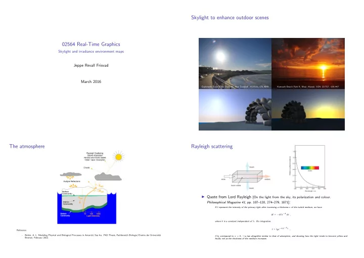
Skylight to enhance outdoor scenes
Esplanade, Saint Clair, Dunedin, New Zealand: -45.9121, 170.4893 Kamaole Beach Park II, Maui, Hawaii, USA: 20.717, -156.447
The atmosphere
Reference
- Bel´
em, A. L. Modeling Physical and Biological Processes in Antarctic Sea Ice. PhD Thesis, Fachbereich Biologie/Chemie der Universit¨ at Bremen, February 2002.
Rayleigh scattering
◮ Quote from Lord Rayleigh [On the light from the sky, its polarization and colour.
Philosophical Magazine 41, pp. 107–120, 274–279, 1871]:
If I represent the intensity of the primary light after traversing a thickness x of the turbid medium, we have dI = −kIλ−4 dx , where k is a constant independent of λ. On integration, I = I0e−kλ−4x , if I0 correspond to x = 0, —a law altogether similar to that of absorption, and showing how the light tends to become yellow and finally red as the thickness of the medium increases.