
SLIDE 1
11/20/2007 1
Lecture 19: Motion
Tuesday, Nov 20
- Review Problem set 3
– Dense stereo matching – Sparse stereo matching Indexing scenes – Indexing scenes
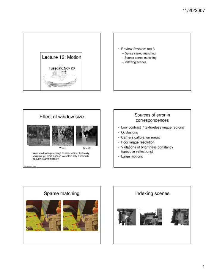
Effect of window size
W = 3 W = 20
Figures from Li Zhang
Want window large enough to have sufficient intensity variation, yet small enough to contain only pixels with about the same disparity.
Sources of error in correspondences
- Low-contrast / textureless image regions
- Occlusions
- Camera calibration errors
Camera calibration errors
- Poor image resolution
- Violations of brightness constancy
(specular reflections)
- Large motions