Signal detection theory z p[r|-] p[r|+] <r> + <r> - - PowerPoint PPT Presentation

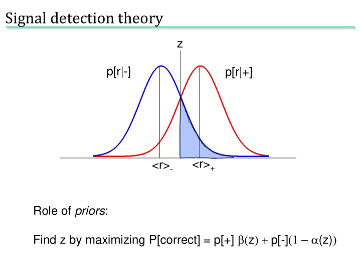
Signal detection theory z p[r|-] p[r|+] <r> + <r> - Role of priors : Find z by maximizing P[correct] = p[+] b( z ) + p[-] (1 – a (z) )

Is there a better test to use than r ? z p[r|-] p[r|+] <r> + <r> - The optimal test function is the likelihood ratio , l(r) = p[r|+] / p[r|-]. (Neyman-Pearson lemma)

Building in cost Penalty for incorrect answer: L + , L - For an observation r, what is the expected loss ? Loss + = L + P[-|r] Loss - = L - P[+|r] Cut your losses: answer + when Loss + < Loss - i.e. when L + P[-|r] < L - P[+|r]. Using Bayes’, P[+|r] = p[r|+]P[+]/p(r); P[-|r] = p[r|-]P[-]/p(r);  l(r) = p[r|+]/p[r|-] > L + P[-] / L - P[+] .

Decoding from many neurons: population codes • Population code formulation • Methods for decoding:  population vector  Bayesian inference  maximum likelihood  maximum a posteriori • Fisher information

Cricket cercal cells

Population vector RMS error in estimate Theunissen & Miller, 1991

Population coding in M1 Cosine tuning: Pop. vector:

Is this the best one can do? The population vector is neither general nor optimal. “Optimal”: make use of all information in the stimulus/response distributions

Bayesian inference Bayes ’ law: likelihood function conditional distribution prior distribution a posteriori distribution marginal distribution

Bayesian estimation Want an estimator s Bayes Introduce a cost function, L(s,s Bayes ); minimize mean cost. For least squares cost, L(s,s Bayes ) = (s – s Bayes ) 2 . Let’s calculate the solution..

Bayesian inference By Bayes ’ law, likelihood function a posteriori distribution

Maximum likelihood Find maximum of p[r|s] over s More generally, probability of the data given the “model” “Model” = stimulus assume parametric form for tuning curve

Bayesian inference By Bayes ’ law, likelihood function a posteriori distribution

MAP and ML ML: s* which maximizes p[r|s] MAP: s* which maximizes p[s|r] Difference is the role of the prior: differ by factor p[s]/p[r]

Comparison with population vector

Decoding an arbitrary continuous stimulus Many neurons “voting” for an outcome. Work through a specific example • assume independence • assume Poisson firing Noise model: Poisson distribution P T [k] = ( l T) k exp(- l T)/k!

Decoding an arbitrary continuous stimulus E.g. Gaussian tuning curves .. what is P(r a |s)?

Need to know full P[ r |s] Assume Poisson: Assume independent: Population response of 11 cells with Gaussian tuning curves

ML Apply ML: maximize ln P[ r |s] with respect to s Set derivative to zero, use sum = constant From Gaussianity of tuning curves, If all s same

MAP Apply MAP: maximise ln p[s| r ] with respect to s Set derivative to zero, use sum = constant From Gaussianity of tuning curves,

Given this data: Prior with mean -2, variance 1 Constant prior MAP:

How good is our estimate? For stimulus s, have estimated s est Bias: Variance: Mean square error: Cramer-Rao bound: Fisher information (ML is unbiased: b = b ’ = 0)

Fisher information Alternatively: Quantifies local stimulus discriminability

Fisher information for Gaussian tuning curves For the Gaussian tuning curves w/Poisson statistics:

Are narrow or broad tuning curves better? Approximate:  Narrow tuning curves are better Thus, But not in higher dimensions! ..what happens in 2D?

Fisher information and discrimination Recall d' = mean difference/standard deviation Can also decode and discriminate using decoded values. Trying to discriminate s and s+ D s: Difference in ML estimate is D s (unbiased) variance in estimate is 1/I F (s). 

Limitations of these approaches • Tuning curve/mean firing rate • Correlations in the population

The importance of correlation Shadlen and Newsome, ‘98

The importance of correlation

The importance of correlation

Entropy and Shannon information Model-based vs model free