Security storage and manufacturing flows subject to random - PDF document
Security storage and manufacturing flows subject to random fluctuations Max-Olivier Hongler EPFL/Laboratoire GALATEA 15 aot 2016 Preliminary consideration A wide set of multidisciplinary skills are required to conceive and control au-
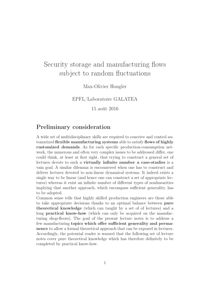
Security storage and manufacturing flows subject to random fluctuations Max-Olivier Hongler EPFL/Laboratoire GALATEA 15 août 2016 Preliminary consideration A wide set of multidisciplinary skills are required to conceive and control au- tomatized flexible manufacturing systems able to satisfy flows of highly customized demands . As for each specific production-consumption net- work, the numerous and often very complex issues to be addressed differ, one could think, at least at first sight, that trying to construct a general set of lectures devote to such a virtually infinite number a case-studies is a vain goal. A similar dilemma is encountered when one has to construct and deliver lectures devoted to non-linear dynamical systems. It indeed exists a single way to be linear (and hence one can construct a set of appropriate lec- tures) whereas it exist an infinite number of different types of nonlinearities implying that another approach, which encompass sufficient generality, has to be adopted. Common sense tells that highly skilled production engineers are those able to take appropriate decisions thanks to an optimal balance between pure theoretical knowledge (which can taught by a set of of lectures) and a long practical know-how (which can only be acquired on the manufac- turing shop-floors). The goal of the present lecture notes is to address a few manufacturing topics which offer sufficient generality and perma- nence to allow a formal theoretical approach that can be exposed in lectures. Accordingly, the potential reader is warned that the following set of lecture notes cover pure theoretical knowledge which has therefore definitely to be completed by practical know-how. 1
1 Optimization issues and random environments Whatever the production-consumption systems to be considered, random fluctuation will ubiquitously affect any idealized picture we always initially start with. On one hand, production systems are practically always failure prone and simultaneously, customers demands (like the types and quantities of finished products) are barely completely predictable. Adopting a highly stylized view, we can generically say that any production system delivers a randomly fluctuating flow of finished goods to cover a randomly fluctuating flow of customers demands. The unavoidable and ubiquitous presence of ran- domness raises a couple of basic engineering questions that we shall address, namely : a) How to enhance the average finished goods flows and how to mini- mize the variability of complex automatized production networks com- posed of failure prone echelons ? (i.e. determine the optimal capa- city of buffers in production lines ). b) How large should be the security stocks required to ensure on-hand delivery to incoming customers, (i.e. determine the optimal capa- city of hedging stocks ). 2 Characterizing the production output of a failure prone machines Let us consider a production station M which delivers a single type of finished parts. In ideal operation condition, the time required to complete a single part is the cycle time τ c ; it therefore has the physical dimension of a time. The inverse of the cycle time U = τ − 1 is the production rate ; it hence c has the physical dimension of a frequency. In the sequel, we shall focus on elementary machines for which both τ c and U are constants. 1 Hence, ideally, the cumulate production S ( T ) delivered during a time time interval [0 , T ] exhibits a step structure, as represented in Figure 1, and reads : 1 Observe that for certain types of production, (like for example fluids in chemistry and/or in food industries), it is possible to pilot the production rate but in the sequel we focus on constant rates. 2
Fig. 1 – Cumulative production for a failure prone production center modeled via an "hydrodynamic" fluid queue picture. N ( T ) � S ( T ) = Θ( T − kτ c ) with N ( t ) := sup { k : kτ c < T, } (1) k =1 where Θ( T − kτ c ) is the Heavyside step function : 1 when T ≥ kτ c , Θ( T − kτ c ) = (2) 0 when T > kτ c . Generally, the station M can be interrupted either deterministically (night breaks for example) or randomly due to unpredictable failures . Accor- dingly, the cumulative production during a time horizon T Eq.(1) has to be modified as : N ( T ) � S ( T ) = Θ( T − kτ c ) χ ( kτ c ) with N ( t ) := sup { k : kτ c < T, } (3) k =1 where the state operating function χ ( t ) = 1 when M is operational at time t and conversely χ ( t ) = 0 when M is out-of-service at t . In the sequel, we shall focus on situations where χ ( t ) models failures. In this case, the operating function χ ( t ) will be a random function which alternates between the 3
values 0 , (when M is OFF) and 1 (when M is ON) and the sojourn time intervals in the states 0 and 1 are random variables (r.v.) (i.e. time intervals having random durations ). In the sequel, we shall always assume that successive alternating cycles 2 are statistically independent. The posotive definite r.v. characterizing the ON time duration t ON ∈ R + is drawn from a probability density f ON ( ζ ) and similarly then r.v. characterizing the OFF time duration t OFF ∈ R + is drawn from a probability density f OFF ( ζ ) and hence, we formally can write : Prob { ζ ≤ t ON ≤ ( ζ + dζ ) } := f ON ( ζ ) dζ, (4) Prob { ζ ≤ t OFF ≤ ( ζ + dζ ) } := f OFF ( ζ ) dζ. For future use, let us now introduce the notations for the first moments of these probability densities. We namely have the average 3 � ∞ 0 ζ f ON ( ζ ) dζ := λ − 1 , E { t ON } := (5) � ∞ 0 ζf OFF ( ζ ) dζ := µ − 1 , E { t OFF } := and similarly the associated variances are defined as : � ∞ ON } − [ E { t ON } ] 2 = 0 ζ 2 f ON ( ζ ) dζ − λ − 2 , σ 2 ON := E { t 2 (6) � ∞ OFF } − [ E { t OFF } ] 2 = σ 2 ON := E { t 2 0 ζ 2 f OFF ( ζ ) dζ − µ − 2 . At this stage, we define the (dimensionless) unavailability factor J as : average time of operation = 1 /µ average time to repair 1 /λ = λ J = µ. (7) We now also introduce the couple of dimensionless (positive definite) coeffi- cients of variations : 4 : CV 2 ON := σ 2 ON λ 2 , (8) CV 2 OFF := σ 2 OFF µ 2 . To proceed further, we shall now distinguish between two modeling frame- works defined by two time scales regimes of the M dynamics : 2 A cycle is formed by a single ON and OFF alternation. 3 The operator E ( Z ) stands for the expectation of the r.v. Z . 4 The coefficient of variation which is a dimensionless factor, is only defined for strictly positive r.v. The CV 2 factor directly measures the strength of the fluctuations. Observe in particular that a r.v. with CV 2 = 0 is effectively an ordinary deterministic quantity. 4
a) Discrete queuing dynamics . This regime occurs when the time inter- vals τ c , λ − 1 and µ − 1 have identical orders of magnitude. In this case, the discrete nature of the production output cannot be ignored and the appropriate theory to model the production output is the classi- cal queuing dynamics . Typical example will be production of cars, engines and most of highly complex devices for which the cycle time is pretty long. b) Fluid queueing dynamics . This regime is characterized by the fact that τ c >> λ − 1 and τ c >> µ − 1 . This characterizes high production flows like those encountered in productions of chocolate, cigarettes, screws and many other simple and usually tiny parts typical in micro- engineering shop-floors. For these regimes, the discrete nature of the production flows almost disappears and we may consider that we effec- tively deal with a fluid of parts for which the appropriate dynamics is known as the fluid queue dynamics . In the sequel, we shall focus on this type of production. 3 The fluid queue approach For high production rate, the production output is assimilable to a fluid flow (like one would view the flow of sand grains in an hour glass). It is interrupted during a random time interval τ ON (i.e when M is OFF) and then restituted to its nominal value after that M has been repaired. The random reparation time is τ OFF . In the fluid approximation, without failure, (i.e. χ ( t ) ≡ 1 ∀ t the cumulative production output S ( t ) is simply an increasing a straight line with slope U . Alternatively, in presence of failure (i.e. χ ( t ) randomly alternates between 0 and 1 ), the cumulative output S ( t ) delivered by M is a random piecewise increasing function (i.e. a time-dependent stochastic process ) as sketched in Figure 2. Let us now characterize the stochastic process S ( t ) . The following proposition can be proved : Proposition 1. 5 For large production time horizon T >> max { λ − 1 , µ − 1 } , the random cumulative production S ( T ) is approximately characterized by 5 The proof of this proposition can be found in the contribution by Ph. Ciprut, M.-O. Hongler and Y. Salama, "On the Variance of the Production Output of Transfer Lines" published in IEEE Trans. on Robotics and Automation 15 , (1999), 33-43. Basically the proof relies on the Central Limit Theorem. 5
Recommend
More recommend
Explore More Topics
Stay informed with curated content and fresh updates.

