The boundary Flows-3 conditions A Simple Solver for Variable - - PDF document

SLIDE 1

DNS of Multiphase Flows Gretar Tryggvason

Direct Numerical Simulations of Multiphase Flows-3
 


A Simple Solver for Variable Density Flow (3 of 3)

DNS of Multiphase Flows

The boundary conditions

DNS of Multiphase Flows Boundary Conditions for the velocity: Here we take the domain to be a rectangle with prescribed velocities at all boundaries. The boundaries coincide with the edges of the pressure control volumes so the normal velocity is given where it is needed. The implementation of the tangent velocity is slightly more complex and we will use “ghost” points outside the domain to impose the correct tangential velocity DNS of Multiphase Flows Velocity of wall is given, uwall (no-slip) Tangent velocity Boundary Conditions Interpolate linearly Solve for the “ghost” velocity If the wall velocity is zero: then the ghost velocity is a reflection of the interior velocity ui,1 = 2 uwall − ui,2 uwall = 0 ui,1 = ui,2

uwall = ui,1 + ui,2 2

pi,2

!

pi+1,2! pi,1! pi+1,1! vi,2! vi+1,2! vi,1! vi+1,1! ui,2! ui,1! % tangential velocity at boundaries u(1:nx+1,1)=2*usouth-u(1:nx+1,2); u(1:nx+1,ny+2)=2*unorth-u(1:nx+1,ny+1); v(1,1:ny+1)=2*vwest-v(2,1:ny+1); v(nx+2,1:ny+1)=2*veast-v(nx+1,1:ny+1);

DNS of Multiphase Flows

pi,j! pi+1,j! vi,j+1/2! vi,j-1/2! vi+1,j+1/2! vi+1,j-1/2! ui+1/2,j! Ub,j = ui-1/2,j!

Boundary Conditions for the

• pressure. Use the normal

velocity given at the boundary when we substitute the correction velocity into the mass conservation equation: The pressure equation at the boundary is therefore:

un+1

i+1/2,j Ub,j

∆x + vn+1

i,j+1/2 vn+1 i,j−1/2

∆y = 0

1 ∆x2 pi+1,j pi,j ρn+1

i+1,j + ρn+1 i,j

! + 1 ∆y2 pi,j+1 pi,j ρn+1

i,j+1 + ρn+1 i,j

pi,j pi,j−1 ρn+1

i,j

+ ρn+1

i,j−1

! = 1 2∆t ⇣u∗

i+1/2,j Ub,j

∆x + v∗

i,j+1/2 v∗ i,j−1/2

∆y ⌘

DNS of Multiphase Flows A simple way to implement the pressure boundary conditions is to set the value of the density in the ghost cell to a large value and the velocity to the normal velocity

rt=r; lrg=1000; rt(1:nx+2,1)=lrg; rt(1:nx+2,ny+2)=lrg; rt(1,1:ny+2)=lrg; rt(nx+2,1:ny+2)=lrg; pα+1

i,j

= β " 1 ∆x2 ⇣ 1 ρn+1

i+1,j + ρn+1 i,j

+ 1 ρn+1

i,j

+ ρn+1

i−1,j

⌘ + 1 ∆y2 ⇣ 1 ρn+1

i,j+1 + ρn+1 i,j

+ 1 ρn+1

i,j

+ ρn+1

i,j−1

⌘#−1 " 1 ∆x2 ⇣ pα

i+1,j

ρn+1

i+1,j + ρn+1 i,j

+ pα+1

i−1,j

ρn+1

i,j

+ ρn+1

i−1,j

⌘ + 1 ∆y2 ⇣ pα

i,j+1

ρn+1

i,j+1 + ρn+1 i,j

+ pα+1

i,j−1

ρn+1

i,j

+ ρn+1

i,j−1

⌘ − 1 2∆t ⇣u∗

i+1/2,j − u∗ i−1/2,j

∆x + v∗

i,j+1/2 − v∗ i,j−1/2

∆y ⌘# + (1 − β)pα

i,j

SLIDE 2

DNS of Multiphase Flows

Advecting the Density

DNS of Multiphase Flows Advecting the Density: Centered Differences with Diffusion Write as: Add a diffusion term Discrete version

∂ρ ∂t = u · rρ ∂ρ ∂t = r · (ρu) ∂ρ ∂t = r · (ρu) + µ0r2ρ ρn+1

i,j

= ρn

i,j ∆t

∆x ⇣ ui+1/2,j ρi+1,j + ρi,j 2 ui−1/2,j ρi−1,j + ρi,j 2 ⌘ ∆t ∆y ⇣ vi,j+1/2 ρi,j+1 + ρi,j 2 ui,j−1/2 ρi,j−1 + ρi,j 2 ⌘ +µ0∆t ∆x2 (ρi+1,j 2ρi,j + ρi−1,j) + µ0∆t ∆y2 (ρi,j+1 2ρi,j + ρi,j−1)

DNS of Multiphase Flows Discrete version

%=====ADVECT DENSITY using centered difference plus diffusion ======== ro=r; for i=2:nx+1,for j=2:ny+1 r(i,j)=ro(i,j)-(0.5*dt/dx)*(u(i,j)*(ro(i+1,j)+ro(i,j))-u(i-1,j)*(ro(i-1,j)+ro(i,j)) )...

• (0.5*dt/dy)*(v(i,j)*(ro(i,j+1)+ro(i,j))-v(i,j-1)*(ro(i,j-1)+ro(i,j)) )...

+(m0*dt/dx/dx)*(ro(i+1,j)-2.0*ro(i,j)+ro(i-1,j))... +(m0*dt/dy/dy)*(ro(i,j+1)-2.0*ro(i,j)+ro(i,j-1)); end,end

ρn+1

i,j

= ρn

i,j ∆t

∆x ⇣ ui+1/2,j ρi+1,j + ρi,j 2 ui−1/2,j ρi−1,j + ρi,j 2 ⌘ ∆t ∆y ⇣ vi,j+1/2 ρi,j+1 + ρi,j 2 ui,j−1/2 ρi,j−1 + ρi,j 2 ⌘ +µ0∆t ∆x2 (ρi+1,j 2ρi,j + ρi−1,j) + µ0∆t ∆y2 (ρi,j+1 2ρi,j + ρi,j−1)

DNS of Multiphase Flows

The full method

DNS of Multiphase Flows

• 2. Find a temporary velocity using the advection and the

diffusion terms only:

• 3. Find the pressure needed to make the velocity

field incompressible

• 4. Correct the velocity by adding the pressure gradient:
• 1. Set velocity at ghost points and update the marker function

to find new density and viscosity Discretization in time

⇣

h h

rh · 1 ρn+1

h

rhph ! = 1 ∆trh · u∗

h

un+1

h

= u∗

h ∆trhph

ρn+1

h

u∗

h =

1 ρn+1

h

ρn

hun h + ∆t

• An

h + gh + Dn h

• !

!

DNS of Multiphase Flows Algorithm Determine u, v boundary conditions Initial field given t=t+Δt

Initialize parameters and arrays, set time step and initial density for is=1:nstep set boundary conditions for tangential velocity (ghost points) Advect the density Find predicted velocity Solve for pressure using SOR Find the projected velocity by adding the pressure gradient PLOT end

Advect density

⇣

h h

rh · 1 ρn+1

h

rhph ! = 1 ∆trh · u∗

h

un+1

h

= u∗

h ∆trhph

ρn+1

h

u∗

h =

1 ρn+1

h

ρn

hun h + ∆t

• An

h + gh + Dn h

• !

!

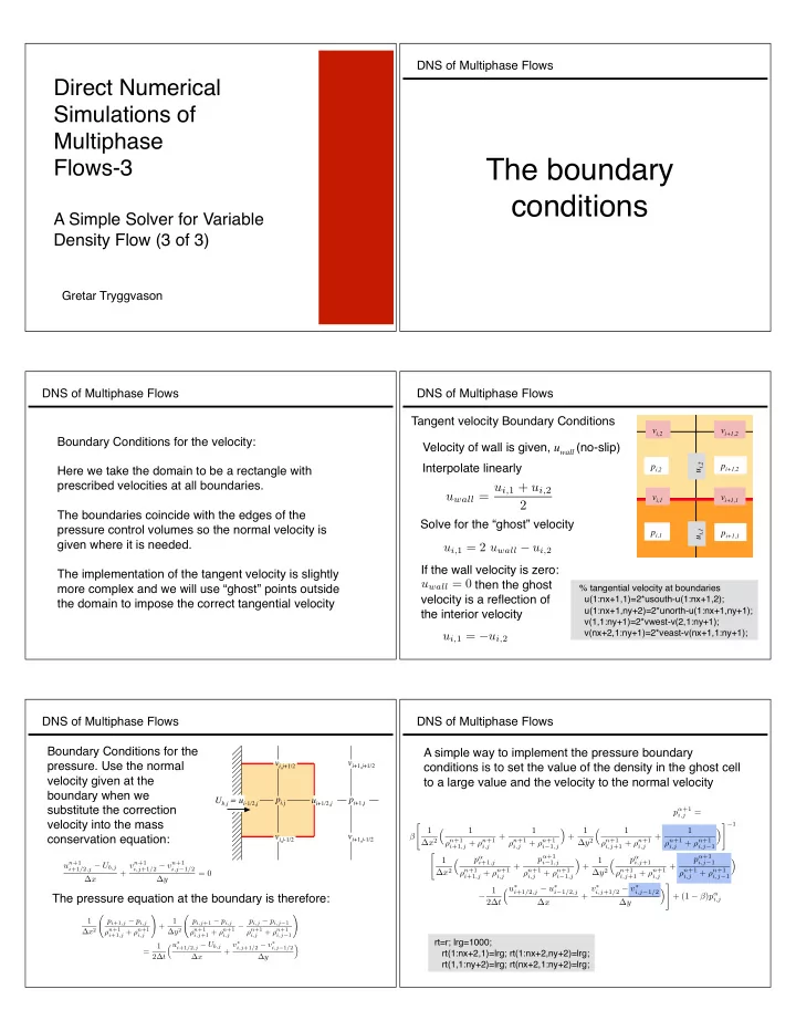
SLIDE 3

DNS of Multiphase Flows

Code

See sample matlab code CodeC1.m

%=================================================================== % A very simple Navier-Stokes solver for a drop falling in a rectangular % domain. The viscosity is taken to be a constant and a forward in time, % and a conservative centered in space discretization is used. The density % is advected by solving a simple advection-diffusion equation. %===================================================================

DNS of Multiphase Flows

for i=2:nx+1,for j=2:ny % TEMPORARY v-velocity vt(i,j)=(2.0/(r(i,j+1)+r(i,j)))*( 0.5*(ro(i,j+1)+ro(i,j))*v(i,j)+ dt* ( ...

• (0.0625/dx)*( (ro(i,j)+ro(i+1,j)+ro(i+1,j+1)+ro(i,j+1))*...

(u(i,j)+u(i,j+1))*(v(i,j)+v(i+1,j)) ...

• (ro(i,j)+ro(i,j+1)+ro(i-1,j+1)+ro(i-1,j))*...

(u(i-1,j+1)+u(i-1,j))*(v(i,j)+v(i-1,j)) ) ...

• (0.25/dy)*(ro(i,j+1)*(v(i,j+1)+v(i,j))^2-ro(i,j)*(v(i,j)+v(i,j-1))^2 ) ...

+ 0.5*(ro(i,j+1)+ro(i,j))*gy ... +m0*((v(i+1,j)-2*v(i,j)+v(i-1,j))/dx^2+(v(i,j+1)-2*v(i,j)+v(i,j-1))/dy^2)) ); end,end %======================================================================== % Compute source term and the coefficient for p(i,j) rt=r; lrg=1000; rt(1:nx+2,1)=lrg;rt(1:nx+2,ny+2)=lrg; rt(1,1:ny+2)=lrg;rt(nx+2,1:ny+2)=lrg; for i=2:nx+1,for j=2:ny+1 tmp1(i,j)= (0.5/dt)*( (ut(i,j)-ut(i-1,j))/dx+(vt(i,j)-vt(i,j-1))/dy ); tmp2(i,j)=1.0/( (1./dx)*( 1./(dx*(rt(i+1,j)+rt(i,j)))+... 1./(dx*(rt(i-1,j)+rt(i,j))) )+... (1./dy)*(1./(dy*(rt(i,j+1)+rt(i,j)))+... 1./(dy*(rt(i,j-1)+rt(i,j))) ) ); end,end for it=1:maxit % SOLVE FOR PRESSURE

• ldArray=p;

for i=2:nx+1,for j=2:ny+1 p(i,j)=(1.0-beta)*p(i,j)+beta* tmp2(i,j)*(... (1./dx)*( p(i+1,j)/(dx*(rt(i+1,j)+rt(i,j)))+... p(i-1,j)/(dx*(rt(i-1,j)+rt(i,j))) )+... (1./dy)*( p(i,j+1)/(dy*(rt(i,j+1)+rt(i,j)))+... p(i,j-1)/(dy*(rt(i,j-1)+rt(i,j))) ) - tmp1(i,j)); end,end if max(max(abs(oldArray-p))) <maxError, break,end end for i=2:nx, for j=2:ny+1 % CORRECT THE u-velocity u(i,j)=ut(i,j)-(dt*2.0/(r(i+1,j)+r(i,j)))*(p(i+1,j)-p(i,j))/dx; end, end for i=2:nx+1, for j=2:ny % CORRECT THE v-velocity v(i,j)=vt(i,j)-(dt*2.0/(r(i,j+1)+r(i,j)))*(p(i,j+1)-p(i,j))/dy; end, end %======================================================================== time=time+dt % plot the results uu(1:nx+1,1:ny+1)=0.5*(u(1:nx+1,2:ny+2)+u(1:nx+1,1:ny+1)); vv(1:nx+1,1:ny+1)=0.5*(v(2:nx+2,1:ny+1)+v(1:nx+1,1:ny+1)); for i=1:nx+1,xh(i)=dx*(i-1);end; for j=1:ny+1,yh(j)=dy*(j-1);end hold off,contour(x,y,flipud(rot90(r))),axis equal,axis([0 Lx 0 Ly]); hold on;quiver(xh,yh,flipud(rot90(uu)),flipud(rot90(vv)),'r'); pause(0.01) end %======================================================================== % CodeC1.m % A very simple Navier-Stokes solver for a drop falling in a rectangular % domain. The viscosity is taken to be a constant and a forward in time, % and a conservative centered in space discretization is used. The density % is advected by solving a simple advection-diffusion equation. %======================================================================== %domain size and physical variables Lx=1.0;Ly=1.0;gx=0.0;gy=-100.0; rho1=1.0; rho2=2.0; m0=0.01; unorth=0;usouth=0;veast=0;vwest=0;time=0.0; rad=0.15;xc=0.5;yc=0.7; % Initial drop size and location % Numerical variables nx=32;ny=32;dt=0.00125;nstep=100; maxit=200;maxError=0.001;beta=1.2; % Zero various arrys u=zeros(nx+1,ny+2); v=zeros(nx+2,ny+1); p=zeros(nx+2,ny+2); ut=zeros(nx+1,ny+2); vt=zeros(nx+2,ny+1); tmp1=zeros(nx+2,ny+2); uu=zeros(nx+1,ny+1); vv=zeros(nx+1,ny+1); tmp2=zeros(nx+2,ny+2); % Set the grid dx=Lx/nx;dy=Ly/ny; for i=1:nx+2; x(i)=dx*(i-1.5);end; for j=1:ny+2; y(j)=dy*(j-1.5);end; % Set density in the domain and the drop r=zeros(nx+2,ny+2)+rho1; for i=2:nx+1,for j=2:ny+1; if ( (x(i)-xc)^2+(y(j)-yc)^2 < rad^2), r(i,j)=rho2;end, end,end %================== START TIME LOOP====================================== for is=1:nstep,is % tangential velocity at boundaries u(1:nx+1,1)=2*usouth-u(1:nx+1,2);u(1:nx+1,ny+2)=2*unorth-u(1:nx+1,ny+1); v(1,1:ny+1)=2*vwest-v(2,1:ny+1);v(nx+2,1:ny+1)=2*veast-v(nx+1,1:ny+1); %=======ADVECT DENSITY using centered difference plus diffusion ========== ro=r; for i=2:nx+1,for j=2:ny+1 r(i,j)=ro(i,j)-(0.5*dt/dx)*(u(i,j)*(ro(i+1,j)... +ro(i,j))-u(i-1,j)*(ro(i-1,j)+ro(i,j)))-(0.5* dt/dy)*(v(i,j)*(ro(i,j+1)... +ro(i,j))-v(i,j-1)*(ro(i,j-1)+ro(i,j)) )... +(m0*dt/dx/dx)*(ro(i+1,j)-2.0*ro(i,j)+ro(i-1,j))... +(m0*dt/dy/dy)*(ro(i,j+1)-2.0*ro(i,j)+ro(i,j-1)); end,end %===== Find temporary velocities ======================================== for i=2:nx,for j=2:ny+1 % TEMPORARY u-velocity ut(i,j)=(2.0/(r(i+1,j)+r(i,j)))* ( 0.5*(ro(i+1,j)+ro(i,j))*u(i,j)+ dt* (...

• (0.25/dx)*(ro(i+1,j)*(u(i+1,j)+u(i,j))^2-ro(i,j)*(u(i,j)+u(i-1,j))^2) ...
• (0.0625/dy)*( (ro(i,j)+ro(i+1,j)+ro(i,j+1)+ro(i+1,j+1))*...

(u(i,j+1)+u(i,j))*(v(i+1,j)+v(i,j)) ...

• (ro(i,j)+ro(i+1,j)+ro(i+1,j-1)+ro(i,j-1))*(u(i,j)...

+u(i,j-1))*(v(i+1,j-1)+v(i,j-1))) ... + 0.5*(ro(i+1,j)+ro(i,j))*gx ... +m0*((u(i+1,j)-2*u(i,j)+u(i-1,j))/dx^2+ (u(i,j+1)-2*u(i,j)+u(i,j-1))/dy^2)) ); end,end

DNS of Multiphase Flows Limitations on the time step where The time step needs to be small enough so that the code is

• stable. For the explicit method used here we need to use:

h = max(∆x, ∆y)

µ∆t ρh2  1 4 (u · u)max ρ∆t µ  2 DNS of Multiphase Flows

Problem specification: Lx=1.0; Ly=1.0; gx=0.0; gy=-100.0; rho1=1.0; rho2=2.0; m0=0.01; Tangential velocities: unorth=0;usouth=0; veast=0;vwest=0; Initial drop size and location rad=0.15; xc=0.5; yc=0.7; Numerical variables nx=32; ny=32; dt=0.00125; nstep=100; Pressure solver maxit=200; beta=1.2; maxError=0.001;

0.2 0.4 0.6 0.8 1 0.2 0.4 0.6 0.8 1 0.8 1 1.2 1.4 1.6 1.8 2 2.2

Example: An initially stationary droplet in a square box that falls down due to gravity. Here we ignore surface tension, take the viscosity to be the same as the ambient fluid and advect density by solving the advection-diffusion equation

DNS of Multiphase Flows

0.1 0.2 0.3 0.4 0.5 0.6 0.7 0.8 0.9 1 0.1 0.2 0.3 0.4 0.5 0.6 0.7 0.8 0.9 1 0.1 0.2 0.3 0.4 0.5 0.6 0.7 0.8 0.9 1 0.1 0.2 0.3 0.4 0.5 0.6 0.7 0.8 0.9 1

time=0.00125 time=0.125

5 10 15 20 25 30 35 10 20 30 40 0.8 1 1.2 1.4 1.6 1.8 2

“Exact” solution

5 10 15 20 25 30 35 10 20 30 40 0.8 1 1.2 1.4 1.6 1.8 2 2.2

Density at final time Numerical results for a falling drop on a 32 by 32 grid