TABLE I S UMMARY S TATISTICS a Sample Falls Within < 100 km of - PowerPoint PPT Presentation

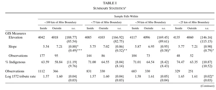
TABLE I S UMMARY S TATISTICS a Sample Falls Within < 100 km of Mita Boundary < 75 km of Mita Boundary < 50 km of Mita Boundary < 25 km of Mita Boundary Inside Outside s.e. Inside Outside s.e. Inside Outside s.e. Inside Outside s.e. GIS Measures Elevation 4042 4018 [ 188 � 77 ] 4085 4103 [ 166 � 92 ] 4117 4096 [ 169 � 45 ] 4135 4060 [ 146 � 16 ] (85 � 54) (82 � 75) (89 � 61) (115 � 15) Slope 5 � 54 7 � 21 [ 0 � 88 ] * 5 � 75 7 � 02 [ 0 � 86 ] 5 � 87 6 � 95 [ 0 � 95 ] 5 � 77 7 � 21 [ 0 � 90 ] (0 � 49)*** (0 � 52)** (0 � 58)* (0 � 79)* Observations 177 95 144 86 104 73 48 52 % Indigenous 63 � 59 58 � 84 [ 11 � 19 ] 71 � 00 64 � 55 [ 8 � 04 ] 71 � 01 64 � 54 [ 8 � 42 ] 74 � 47 63 � 35 [ 10 � 87 ] (9 � 76) (8 � 14) (8 � 43) (10 � 52) Observations 1112 366 831 330 683 330 329 251 Log 1572 tribute rate 1 � 57 1 � 60 [ 0 � 04 ] 1 � 57 1 � 60 [ 0 � 04 ] 1 � 58 1 � 61 [ 0 � 05 ] 1 � 65 1 � 61 [ 0 � 02 ] * (0 � 03) (0 � 03) (0 � 04) (0 � 03) ( Continues )

TABLE I— Continued Sample Falls Within < 100 km of Mita Boundary < 75 km of Mita Boundary < 50 km of Mita Boundary < 25 km of Mita Boundary Inside Outside s.e. Inside Outside s.e. Inside Outside s.e. Inside Outside s.e. % 1572 tribute to Spanish Nobility 59 � 80 63 � 82 [ 1 � 39 ] *** 59 � 98 63 � 69 [ 1 � 56 ] ** 62 � 01 63 � 07 [ 1 � 12 ] 61 � 01 63 � 17 [ 1 � 58 ] (1 � 36)*** (1 � 53)** (1 � 34) (2 � 21) Spanish Priests 21 � 05 19 � 10 [ 0 � 90 ] ** 21 � 90 19 � 45 [ 1 � 02 ] ** 20 � 59 19 � 93 [ 0 � 76 ] 21 � 45 19 � 98 [ 1 � 01 ] (0 � 94)** (1 � 02)** (0 � 92) (1 � 33) Spanish Justices 13 � 36 12 � 58 [ 0 � 53 ] 13 � 31 12 � 46 [ 0 � 65 ] 12 � 81 12 � 48 [ 0 � 43 ] 13 � 06 12 � 37 [ 0 � 56 ] (0 � 48)* (0 � 60) (0 � 55) (0 � 79) Indigenous Mayors 5 � 67 4 � 40 [ 0 � 78 ] 4 � 55 4 � 29 [ 0 � 26 ] 4 � 42 4 � 47 [ 0 � 34 ] 4 � 48 4 � 42 [ 0 � 29 ] (0 � 85) (0 � 29) (0 � 33) (0 � 39) Observations 63 41 47 37 35 30 18 24 a The unit of observation is 20 × 20 km grid cells for the geospatial measures, the household for % indigenous, and the district for the 1572 tribute data. Conley standard errors for the difference in means between mita and non- mita observations are in brackets. Robust standard errors for the difference in means are in parentheses. For % indigenous, the robust standard errors are corrected for clustering at the district level. The geospatial measures are calculated using elevation data at 30 arc second (1 km) resolution (SRTM (2000)). The unit of measure for elevation is 1000 meters and for slope is degrees. A household is indigenous if its members primarily speak an indigenous language in the home (ENAHO (2001)). The tribute data are taken from Miranda (1583). In the first three columns, the sample includes only observations located less than 100 km from the mita boundary, and this threshold is reduced to 75, 50, and finally 25 km in the succeeding columns. Coefficients that are significantly different from zero are denoted by the following system: *10%, **5%, and ***1%.

F IGURE 2.—Plots of various outcomes against longitude and latitude. See the text for a de- tailed description.

TABLE III S PECIFICATION T ESTS a Dependent Variable Log Equiv. Hausehold Consumption (2001) Stunted Growth, Children 6–9 (2005) Sample Within: < 100 km < 75 km < 50 km < 100 km < 75 km < 50 km Border of Bound. of Bound. of Bound. of Bound. of Bound. of Bound. District (1) (2) (3) (4) (5) (6) (7) Alternative Functional Forms for RD Polynomial: Baseline I Linear polynomial in latitude and longitude Mita − 0 � 294*** − 0 � 199 − 0 � 143 0 � 064*** 0 � 054** 0 � 062** 0 � 068** (0 � 092) (0 � 126) (0 � 128) (0 � 021) (0 � 022) (0 � 026) (0 � 031) Quadratic polynomial in latitude and longitude Mita − 0 � 151 − 0 � 247 − 0 � 361 0 � 073* 0 � 091** 0 � 106** 0 � 087** (0 � 189) (0 � 209) (0 � 216) (0 � 040) (0 � 043) (0 � 047) (0 � 041) Quartic polynomial in latitude and longitude Mita − 0 � 392* − 0 � 324 − 0 � 342 0 � 073 0 � 072 0 � 057 0 � 104** (0 � 225) (0 � 231) (0 � 260) (0 � 056) (0 � 050) (0 � 048) (0 � 042) Alternative Functional Forms for RD Polynomial: Baseline II Linear polynomial in distance to Potosí − 0 � 297*** − 0 � 273*** − 0 � 220** 0 � 050** 0 � 048** 0 � 049** 0 � 071** Mita (0 � 079) (0 � 093) (0 � 092) (0 � 022) (0 � 022) (0 � 024) (0 � 031) Quadratic polynomial in distance to Potosí Mita − 0 � 345*** − 0 � 262*** − 0 � 309*** 0 � 072*** 0 � 064*** 0 � 072*** 0 � 060* (0 � 086) (0 � 095) (0 � 100) (0 � 023) (0 � 022) (0 � 023) (0 � 032) Quartic polynomial in distance to Potosí Mita − 0 � 331*** − 0 � 310*** − 0 � 330*** 0 � 078*** 0 � 075*** 0 � 071*** 0 � 053* (0 � 086) (0 � 100) (0 � 097) (0 � 021) (0 � 020) (0 � 021) (0 � 031) Interacted linear polynomial in distance to Potosí Mita − 0 � 307*** − 0 � 280*** − 0 � 227** 0 � 051** 0 � 048** 0 � 043* 0 � 076*** (0 � 092) (0 � 094) (0 � 095) (0 � 022) (0 � 021) (0 � 022) (0 � 029) Interacted quadratic polynomial in distance to Potosí Mita − 0 � 264*** − 0 � 177* − 0 � 285** 0 � 033 0 � 027 0 � 039* 0 � 036 (0 � 087) (0 � 096) (0 � 111) (0 � 024) (0 � 023) (0 � 023) (0 � 024) ( Continues )

TABLE III— Continued Dependent Variable Log Equiv. Hausehold Consumption (2001) Stunted Growth, Children 6–9 (2005) Sample Within: < 100 km < 75 km < 50 km < 100 km < 75 km < 50 km Border of Bound. of Bound. of Bound. of Bound. of Bound. of Bound. District (1) (2) (3) (4) (5) (6) (7) Alternative Functional Forms for RD Polynomial: Baseline III Linear polynomial in distance to mita boundary Mita − 0 � 299*** − 0 � 227** − 0 � 223** 0 � 072*** 0 � 060*** 0 � 058** 0 � 056* (0 � 082) (0 � 089) (0 � 091) (0 � 024) (0 � 022) (0 � 023) (0 � 032) Quadratic polynomial in distance to mita boundary Mita − 0 � 277*** − 0 � 227** − 0 � 224** 0 � 072*** 0 � 060*** 0 � 061*** 0 � 056* (0 � 078) (0 � 089) (0 � 092) (0 � 023) (0 � 022) (0 � 023) (0 � 030) Quartic polynomial in distance to mita boundary Mita − 0 � 251*** − 0 � 229** − 0 � 246*** 0 � 073*** 0 � 064*** 0 � 063*** 0 � 055* (0 � 078) (0 � 089) (0 � 088) (0 � 023) (0 � 022) (0 � 023) (0 � 030) Interacted linear polynomial in distance to mita boundary − 0 � 301* − 0 � 277 − 0 � 385* 0 � 082 0 � 087 0 � 095 0 � 132** Mita (0 � 174) (0 � 190) (0 � 210) (0 � 054) (0 � 055) (0 � 065) (0 � 053) Interacted quadratic polynomial in distance to mita boundary Mita − 0 � 351 − 0 � 505 − 0 � 295 0 � 140* 0 � 132 0 � 136 0 � 121* (0 � 260) (0 � 319) (0 � 366) (0 � 082) (0 � 084) (0 � 086) (0 � 064) Ordinary Least Squares Mita − 0 � 294*** − 0 � 288*** − 0 � 227** 0 � 057** 0 � 048* 0 � 049* 0 � 055* (0 � 083) (0 � 089) (0 � 090) (0 � 025) (0 � 024) (0 � 026) (0 � 031) Geo. controls yes yes yes yes yes yes yes Boundary F.E.s yes yes yes yes yes yes yes Clusters 71 60 52 289 239 185 63 Observations 1478 1161 1013 158,848 115,761 100,446 37,421 a Robust standard errors, adjusted for clustering by district, are in parentheses. All regressions include geographic controls and boundary segment fixed effects (F.E.s). Columns 1–3 include demographic controls for the number of in- fants, children, and adults in the household. Coefficients significantly different from zero are denoted by the following system: *10%, **5%, and ***1%.