Schedule Date Day Class Title Chapters HW Lab Exam No. Due - - PowerPoint PPT Presentation

ECEN 301 Discussion #16 – Frequency Response 1

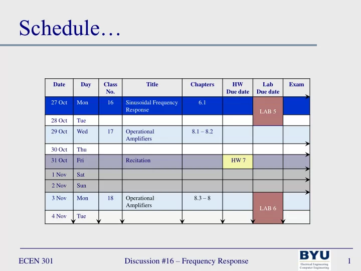
Date Day Class No. Title Chapters HW Due date Lab Due date Exam 27 Oct Mon 16 Sinusoidal Frequency Response 6.1 LAB 5 28 Oct Tue 29 Oct Wed 17 Operational Amplifiers 8.1 – 8.2 30 Oct Thu 31 Oct Fri Recitation HW 7 1 Nov Sat 2 Nov Sun 3 Nov Mon 18 Operational Amplifiers 8.3 – 8 LAB 6 4 Nov Tue Exam 1

Schedule…

ECEN 301 Discussion #16 – Frequency Response 2

Easier to Maintain Than to Retake

Alma 59:9 9 And now as Moroni had supposed that there should be men sent to the city of Nephihah, to the assistance

• f the people to maintain that city, and knowing that it

was easier to keep the city from falling into the hands of the Lamanites than to retake it from them, he supposed that they would easily maintain that city.

ECEN 301 Discussion #16 – Frequency Response 3

Lecture 16 – Frequency Response

Back to AC Circuits and Phasors

• Frequency Response
• Filters

ECEN 301 Discussion #16 – Frequency Response 4

Frequency Response

Frequency Response H(jω): a measure of how the voltage/current/impedance of a load responds to the voltage/current of a source

) ( ) ( ) (    j V j V j H

S L V

 ) ( ) ( ) (    j I j I j H

S L I

 ) ( ) ( ) (    j I j V j H

S L Z



ECEN 301 Discussion #16 – Frequency Response 5

Frequency Response

VL(jω) is a phase-shifted and amplitude-scaled version of VS(jω)

) ( ) ( ) ( ) ( ) ( ) (       j V j H j V j H j V j V

S V L V S L

 

ECEN 301 Discussion #16 – Frequency Response 6

Frequency Response

VL(jω) is a phase-shifted and amplitude-scaled version of VS(jω)

) (

) ( ) ( ) ( ) ( ) ( ) (

S V L S V L

V H j S V j L V j S H j V j L S V L V S L

e V H e V e V e H e V j V j H j V j H j V j V

    

   

 

     

S V L

V H V 

S V L

V H     

A A A e A A

A j

  



as expressed be can number complex any : A NB Amplitude scaled Phase shifted

ECEN 301 Discussion #16 – Frequency Response 7

Frequency Response

Example1: compute the frequency response HV(jω)

R1 = 1kΩ, RL = 10kΩ, C = 10uF

R1 C

vs(t)

+ – + RL –

ECEN 301 Discussion #16 – Frequency Response 8

Frequency Response

Example1: compute the frequency response HV(jω)

R1 = 1kΩ, RL = 10kΩ, C = 10uF

R1 C

vs(t)

+ – + RL – 1. Note frequencies of AC sources Only one AC source so frequency response HV(jω) will be the function of a single frequency

ECEN 301 Discussion #16 – Frequency Response 9

Frequency Response

Example1: compute the frequency response HV(jω)

R1 = 1kΩ, RL = 10kΩ, C = 10uF

R1 C

vs(t)

+ – + RL – 1. Note frequencies of AC sources 2. Convert to phasor domain Z1 = R1 ZLD=RL ZC=1/jωC

Vs

+ – ~

ECEN 301 Discussion #16 – Frequency Response 10

Frequency Response

Example1: compute the frequency response HV(jω)

R1 = 1kΩ, RL = 10kΩ, C = 10uF

1. Note frequencies of AC sources 2. Convert to phasor domain 3. Solve using network analysis

• Thévenin equivalent

Z1 = R1 ZC=1/jωC

C T

Z Z Z ||

1



ECEN 301 Discussion #16 – Frequency Response 11

Frequency Response

Example1: compute the frequency response HV(jω)

R1 = 1kΩ, RL = 10kΩ, C = 10uF

C C S T

Z Z Z j V j V  

1

) ( ) (  

1. Note frequencies of AC sources 2. Convert to phasor domain 3. Solve using network analysis

• Thévenin equivalent

Z1 = R1 + VT – ZC=1/jωC

Vs

+ – ~ C T

Z Z Z ||

1



ECEN 301 Discussion #16 – Frequency Response 12

Frequency Response

Example1: compute the frequency response HV(jω)

R1 = 1kΩ, RL = 10kΩ, C = 10uF

C C S T

Z Z Z j V j V  

1

) ( ) (  

1. Note frequencies of AC sources 2. Convert to phasor domain 3. Solve using network analysis

• Thévenin equivalent

4. Find an expression for the load voltage

C T

Z Z Z ||

1



ZT ZLD

VT

+ – ~ + VL –

 

LD C LD C C S LD T LD T L

Z Z Z Z Z Z Z j V Z Z Z j V j V              || ) ( ) ( ) (

1 1

  

ECEN 301 Discussion #16 – Frequency Response 13

Frequency Response

Example1: compute the frequency response HV(jω)

R1 = 1kΩ, RL = 10kΩ, C = 10uF

5. Find an expression for the frequency response ZT ZLD

VT

+ – ~ + VL –

 

LD C LD C C S L V

Z Z Z Z Z Z Z j V j V j H      || ) ( ) ( ) (

1 1

  

ECEN 301 Discussion #16 – Frequency Response 14

Frequency Response

Example1: compute the frequency response HV(jω)

R1 = 1kΩ, RL = 10kΩ, C = 10uF

5. Find an expression for the frequency response ZT ZLD

VT

+ – ~ + VL –

   

 

                        

  

110 arctan 110 100 110 100 ) 10 /( 10 ) 10 /( 1 10 10 ) 10 /( 10 || ) (

2 2 5 3 5 3 4 5 4 1 1 1 1

       j j j j Z Z Z Z Z Z Z Z Z Z Z Z Z Z j H

C C LD C LD LD C LD C C V

ECEN 301 Discussion #16 – Frequency Response 15

Frequency Response

Example1: compute the frequency response HV(jω)

R1 = 1kΩ, RL = 10kΩ, C = 10uF 2 010 . ) (      j HV

5. Find an expression for the frequency response

• Look at response for low frequencies (ω = 10)

and high frequencies (ω = 10000) ZT ZLD

VT

+ – ~ + VL –

          110 arctan 110 100 ) (

2 2

   j HV

0907 . 905 . ) (     j HV

ω = 10 ω = 10000

ECEN 301 Discussion #16 – Frequency Response 16

Frequency Response

Example2: compute the frequency response HZ(jω)

R1 = 1kΩ, RL = 4kΩ, L = 2mH

R1

is(t)

+ RL – L

ECEN 301 Discussion #16 – Frequency Response 17

Frequency Response

Example2: compute the frequency response HZ(jω)

R1 = 1kΩ, RL = 4kΩ, L = 2mH

R1

is(t)

+ RL – L 1. Note frequencies of AC sources Only one AC source so frequency response HZ(jω) will be the function of a single frequency

ECEN 301 Discussion #16 – Frequency Response 18

Frequency Response

Example2: compute the frequency response HZ(jω)

R1 = 1kΩ, RL = 4kΩ, L = 2mH

R1

is(t)

+ RL – L 1. Note frequencies of AC sources 2. Convert to phasor domain

Is(jω)

ZLD = RL ZL = jωL Z1=R1 + VL –

ECEN 301 Discussion #16 – Frequency Response 19

Frequency Response

Example2: compute the frequency response HZ(jω)

R1 = 1kΩ, RL = 4kΩ, L = 2mH

LD LD L LD L S LD L L

Z Z Z Z Z Z j I Z j I j V             ) ( ) ( || ) ( ) ( ) (

1

  

1. Note frequencies of AC sources 2. Convert to phasor domain 3. Solve using network analysis

• Current divider & Ohm’s Law

Is(jω)

ZLD = RL ZL = jωL Z1=R1 + VL – IL(jω)

) ( ) ( || ) ( ) (

1 LD L LD L S L

Z Z Z Z Z j I j I     

ECEN 301 Discussion #16 – Frequency Response 20

Frequency Response

Example2: compute the frequency response HZ(jω)

R1 = 1kΩ, RL = 4kΩ, L = 2mH

6 1 1 1

10 4 . 1 800 / / 1 ) ( ) ( || ) ( ) ( ) (



               j R L j R R R Z Z Z Z Z Z j I j V j H

L L LD LD L LD L S L Z

Is(jω)

ZLD = RL ZL = jωL Z1=R1 + VL – IL(jω) 4. Find an expression for the frequency response

ECEN 301 Discussion #16 – Frequency Response 21

Frequency Response

Example2: compute the frequency response HZ(jω)

R1 = 1kΩ, RL = 4kΩ, L = 2mH

6

10 4 . 1 800 ) (



     j j HZ

Is(jω)

ZLD = RL ZL = jωL Z1=R1 + VL – IL(jω) 4. Find an expression for the frequency response

• Look at response for low frequencies (ω = 10)

and high frequencies (ω = 10000)

. 4 800 ) (     j HZ

0040 . 800 ) (     j HZ

ω = 10 ω = 10000

ECEN 301 Discussion #16 – Frequency Response 22

1st and 2nd Order RLC Filters

Graphing in Frequency Domain Filter Orders Resonant Frequencies Basic Filters

ECEN 301 Discussion #16 – Frequency Response 23

Frequency Domain

Graphing in the frequency domain: helpful in order to understand filters

• 1.5

0.0 1.5 0.00 2.00 4.00

time x(t)

0.00 3.50

• 600.0

0.0 600.0 w X(jw)

• ω

ω π π

cos(ω0t)

π[δ(ω – ω0) + δ(ω – ω0)]

Time domain Frequency domain

ECEN 301 Discussion #16 – Frequency Response 24

Frequency Domain

Graphing in the frequency domain: helpful in order to understand filters

0.0

• 10.00

0.00 10.00 w X(jw)

• W

W 1

sinc(ω0t)

Time domain Frequency domain

• 0.5
• 10.00

0.00 10.00 t x(t)

W/π π/W

      W W j X | | , | | , 1 ) (   

ECEN 301 Discussion #16 – Frequency Response 25

Electromagnetic (Frequency) Spectrum

ECEN 301 Discussion #16 – Frequency Response 26

Basic Filters

Electric circuit filter: attenuates (reduces) or eliminates signals at unwanted frequencies

0.0

.

Low-pass

0.0

.

High-pass

0.0

.

Band-pass

0.0

.

Band-stop ω ω ω ω

ECEN 301 Discussion #16 – Frequency Response 27

Filter Orders

Higher filter orders provide a higher quality filter

• 150
• 130
• 110
• 90
• 70
• 50
• 30
• 10

10 30 50 0.1 1 10 100 Frequency (w) Gain (dB) 1st Order 2nd Order 3rd Order 4th Order 32nd Order

ECEN 301 Discussion #13 – Phasors 28

Impedance

L j j ZL    ) (

R j ZR  ) ( 

+ L – + C – Re Im

• π/2

π/2 R

• 1/ωC

ωL

ZR ZC ZL

Phasor domain + R –

C j j ZC   1 ) ( 

Vs(jω)

+ – ~ + VZ(jω) – I(jω) Z

Impedance of resistors, inductors, and capacitors

ECEN 301 Discussion #13 – Phasors 29

Impedance

+ C – Re Im

• π/2
• 1/ωC

ZC

C j j ZC   1 ) ( 

Impedance of capacitors

    1 ) ( as   j ZC

+ C –

1 ) ( as        j ZC

+ C –

ECEN 301 Discussion #13 – Phasors 30

Impedance

L j j ZL    ) (

+ L – Re Im π/2 ωL

ZL

Impedance of inductors

) ( as     j ZC

+ L – + L –

    ) ( as   j ZC

ECEN 301 Discussion #16 – Frequency Response 31

Resonant Frequency

Resonant Frequency (ωn): the frequency at which capacitive impedance and inductive impedance are equal and opposite (in 2nd order filters)

LC

n

1  

C + vi(t) – + vo(t) – L C + vi(t) – + vo(t) – L Impedances in series Impedances in parallel

C j L j j Z j Z

C L

    1 ) ( ) (    

ECEN 301 Discussion #16 – Frequency Response 32

Resonant Frequency

Resonant Frequency (ωn): the frequency at which capacitive impedance and inductive impedance are equal and opposite (in 2nd order filters)

C LC j LC LC jL LC LC L LC j L LC j L j Z L                           1 1  ZL=jωL + Vi(jω) – + Vo(jω) – ZC=1/jωC C LC j jC LC C LC j C j ZC            1 / 1 / 1 

Impedances in series

ECEN 301 Discussion #16 – Frequency Response 33

Resonant Frequency

Resonant Frequency (ωn): the frequency at which capacitive impedance and inductive impedance are equal and opposite (in 2nd order filters)

) (   j Vo

C LC j ZL 

+ Vi(jω) – + Vo(jω) – ZEQ=0

C LC j ZC  

  

C L EQ

Z Z Z

Impedances in series

ECEN 301 Discussion #16 – Frequency Response 34

Resonant Frequency

Resonant Frequency (ωn): the frequency at which capacitive impedance and inductive impedance are equal and opposite (in 2nd order filters)

C LC j LC LC jL LC LC L LC j L LC j L j Z L                           1 1  C LC j jC LC C LC j C j ZC            1 / 1 / 1 

Impedances in parallel

ZL=jωL + Vi(jω) – + Vo(jω) – ZC=1/jωC

ECEN 301 Discussion #16 – Frequency Response 35

Resonant Frequency

Resonant Frequency (ωn): the frequency at which capacitive impedance and inductive impedance are equal and opposite (in 2nd order filters)

) ( ) (   j V j V

i

• 

C LC j ZL 

+ Vi(jω) – + Vo(jω) – ZEQ=∞

C LC j ZC  

      / || C L Z Z Z Z Z Z Z

C L C L C L EQ

Impedances in parallel

ECEN 301 Discussion #16 – Frequency Response 36

Low-Pass Filters

Low-pass Filters: only allow signals under the cutoff frequency (ω0) to pass

) cos( ) (

1t

t vo  

0.0

.

Low-pass ω1 ω0 ω2 ω3 ) cos( ) cos( ) cos( ) (

3 2 1

t t t t vi      

HL(jω)

R C + vi(t) – + vo(t) – R C + vi(t) – + vo(t) – L 1st Order 2nd Order

ECEN 301 Discussion #16 – Frequency Response 37

Low-Pass Filters

1st Order Low-pass Filters:

) (  t vo

ZR + Vi(jω) – + Vo(jω) – ZC=1/jωC ZR + Vi(jω) – + Vo(jω) – ω1: ω → 0 ω3: ω → ∞

) ( ) ( t v t v

i

• 

0.0

.

Low-pass ω1 ω0 ω3 ZR + Vi(jω) – + Vo(jω) –

ECEN 301 Discussion #16 – Frequency Response 38

Low-Pass Filters

2nd Order Low-pass Filters:

ZR + Vi(jω) – + Vo(jω) – ZC=1/jωC ZL=jωL ω1: ω → 0

) ( ) ( t v t v

i

• 

ZR + Vi(jω) – + Vo(jω) – ω2: ω = ωn

) (  t vo

ω3: ω → ∞

) (  t vo

ZR + Vi(jω) – + Vo(jω) –

0.0

.

Low-pass ω1 ω0 ω2 ω3 ZR + Vi(jω) – + Vo(jω) –

Resonant frequency

ECEN 301 Discussion #16 – Frequency Response 39

High-Pass Filters

High-pass Filters: only allow signals above the cutoff frequency (ω0) to pass

) cos( ) (

3t

t vo  

) cos( ) cos( ) cos( ) (

3 2 1

t t t t vi      

HH(jω)

0.0

.

High-pass ω1 ω0 ω2 ω3 + vi(t) – + vo(t) – 1st Order R C R + vi(t) – + vo(t) – 2nd Order C L

ECEN 301 Discussion #16 – Frequency Response 40

High-Pass Filters

1st Order High-pass Filters:

) ( ) ( t v t v

i

• 

ZC=1/jωC + Vi(jω) – + Vo(jω) – ZR=R ZR + Vi(jω) – + Vo(jω) – ω1: ω → 0 ω3: ω → ∞

) (  t vo

0.0

.

High-pass ω1 ω0 ω3 ZR + Vi(jω) – + Vo(jω) –

ECEN 301 Discussion #16 – Frequency Response 41

High-Pass Filters

2nd Order High-pass Filters:

ZR + Vi(jω) – + Vo(jω) – ZC=1/jωC ZL=jωL ω1: ω → 0

) (  t vo

ω2: ω = ωn

) (  t vo

ω3: ω → ∞

) ( ) ( t v t v

i

• 

ZR + Vi(jω) – + Vo(jω) –

0.0

.

High-pass ω1 ω0 ω2 ω3 ZR + Vi(jω) – + Vo(jω) – ZR + Vi(jω) – + Vo(jω) –

Resonant frequency

ECEN 301 Discussion #16 – Frequency Response 42

Band-Pass Filters

Band-pass Filters: only allow signals between the passband (ωa to ωb) to pass

) cos( ) (

2t

t vo  

) cos( ) cos( ) cos( ) (

3 2 1

t t t t vi      

HB(jω)

0.0

.

Band-pass ω1 ωa ω2 ω3 ωb + vi(t) – + vo(t) – 2nd Order R C L

ECEN 301 Discussion #16 – Frequency Response 43

Band-Pass Filters

2nd Order Band-pass Filters:

ZR + Vi(jω) – + Vo(jω) – ZC=1/jωC ZL=jωL ω1: ω → 0

) (  t vo

ω2: ω = ωn

) ( ) ( t v t v

i

• 

ω3: ω → ∞

) (  t vo

0.0

.

Band-pass ω1 ωa ω2 ω3 ωb ZR + Vi(jω) – + Vo(jω) – + Vi(jω) – ZR + Vo(jω) – ZR + Vi(jω) – + Vo(jω) –

Resonant frequency

ECEN 301 Discussion #16 – Frequency Response 44

Band-Stop Filters

Band-stop Filters: allow signals except those between the passband (ωa to ωb) to pass

) cos( ) cos( ) (

3 1

t t t vo    

) cos( ) cos( ) cos( ) (

3 2 1

t t t t vi      

HN(jω)

+ vi(t) – + vo(t) – 2nd Order R C L

0.0

.

Band-stop ω1 ωa ω2 ω3 ωb

ECEN 301 Discussion #16 – Frequency Response 45

Band-Stop Filters

2nd Order Band-stop Filters:

ω1: ω → 0

) ( ) ( t v t v

i

• 

ω2: ω = ωn

) (  t vo

ω3: ω → ∞

) ( ) ( t v t v

i

• 

ZR + Vi(jω) – + Vo(jω) – ZC=1/jωC ZL=jωL

0.0

.

Band-stop ω1 ωa ω2 ω3 ωb ZR + Vi(jω) – + Vo(jω) – ZR + Vi(jω) – + Vo(jω) – ZR + Vi(jω) – + Vo(jω) –

Resonant frequency