
SLIDE 1
Discrete-Time Systems
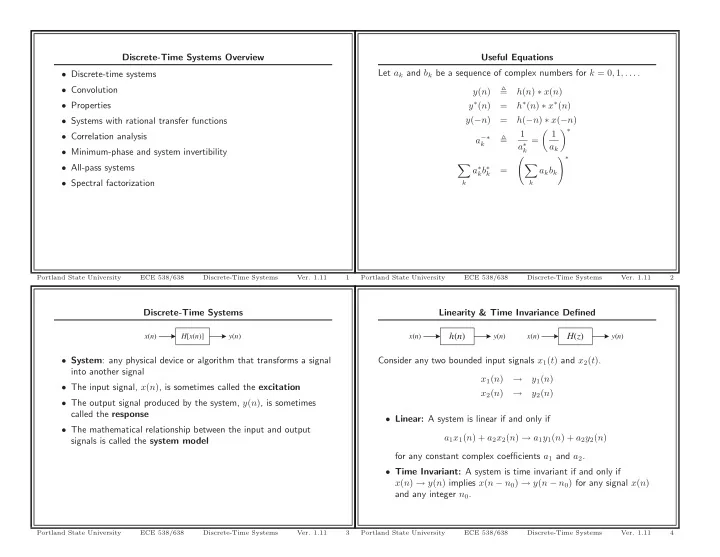
H[x(n)] x(n) y(n)
- System: any physical device or algorithm that transforms a signal
into another signal
- The input signal, x(n), is sometimes called the excitation
- The output signal produced by the system, y(n), is sometimes
called the response
- The mathematical relationship between the input and output
signals is called the system model
Portland State University ECE 538/638 Discrete-Time Systems
- Ver. 1.11
3
Discrete-Time Systems Overview
- Discrete-time systems
- Convolution
- Properties
- Systems with rational transfer functions
- Correlation analysis
- Minimum-phase and system invertibility
- All-pass systems
- Spectral factorization
Portland State University ECE 538/638 Discrete-Time Systems
- Ver. 1.11
1
Linearity & Time Invariance Defined h(n)
x(n) y(n)
H(z)
x(n) y(n)
Consider any two bounded input signals x1(t) and x2(t). x1(n) → y1(n) x2(n) → y2(n)
- Linear: A system is linear if and only if
a1x1(n) + a2x2(n) → a1y1(n) + a2y2(n) for any constant complex coefficients a1 and a2.
- Time Invariant: A system is time invariant if and only if
x(n) → y(n) implies x(n − n0) → y(n − n0) for any signal x(n) and any integer n0.
Portland State University ECE 538/638 Discrete-Time Systems
- Ver. 1.11
4
Useful Equations Let ak and bk be a sequence of complex numbers for k = 0, 1, . . . . y(n)
- h(n) ∗ x(n)
y∗(n) = h∗(n) ∗ x∗(n) y(−n) = h(−n) ∗ x(−n) a−∗
k
- 1
a∗
k
= 1 ak ∗
- k
a∗
kb∗ k
=
- k
akbk ∗
Portland State University ECE 538/638 Discrete-Time Systems
- Ver. 1.11