Road Map Robert Gallagers Minimum Delay Routing Algorithm Using - PowerPoint PPT Presentation

Road Map Robert Gallager’s Minimum Delay Routing Algorithm Using Introduction 1 Distributed Computation Model 2 Timo Bingmann and Dimitar Yordanov Algorithm 3 Decentralized Systems and Network Services Research Group Institute of Telematics, Universität Karlsruhe Conclusion January 29, 2007 4 Timo Bingmann and Dimitar Yordanov - 1 Timo Bingmann and Dimitar Yordanov - 2 Universität Karlsruhe (TH), Winter 2006/07 Universität Karlsruhe (TH), Winter 2006/07 Net Fundamentals Seminar Net Fundamentals Seminar 1 Introduction 1.1 Routing Algorithms 1 Introduction 1.1 Routing Algorithms 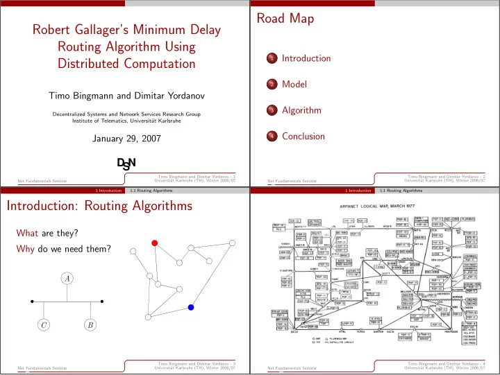Introduction: Routing Algorithms What are they? Why do we need them? A • • C B Timo Bingmann and Dimitar Yordanov - 3 Timo Bingmann and Dimitar Yordanov - 4 Net Fundamentals Seminar Universität Karlsruhe (TH), Winter 2006/07 Net Fundamentals Seminar Universität Karlsruhe (TH), Winter 2006/07

1 Introduction 1.1 Routing Algorithms 1 Introduction 1.1 Routing Algorithms Goals of Routing Algorithms Characteristics Primary Goal Achieve “good” or even optimal routing . How to measure routing quality? Route Calculation Time → Routing metrics Static routing algorithms Other Aims Dynamic routing algorithms little network overhead Quasi-static routing algorithms stability and reliablity adapt to changes quickly converge to optimal state scale well Timo Bingmann and Dimitar Yordanov - 5 Timo Bingmann and Dimitar Yordanov - 6 Universität Karlsruhe (TH), Winter 2006/07 Universität Karlsruhe (TH), Winter 2006/07 Net Fundamentals Seminar Net Fundamentals Seminar 1 Introduction 1.1 Routing Algorithms 2 Model 2.1 Model Development Characteristics Model Other Characteristics Single-Path vs. Multi-Path Algorithms Centralized vs. Distributed Algorithms User vs. System Optimization Timo Bingmann and Dimitar Yordanov - 7 Timo Bingmann and Dimitar Yordanov - 8 Net Fundamentals Seminar Universität Karlsruhe (TH), Winter 2006/07 Net Fundamentals Seminar Universität Karlsruhe (TH), Winter 2006/07

2 Model 2.1 Model Development 2 Model 2.1 Model Development Model Model k k j j r i ( j )+ r l ( j ) i r i ( j ) i l l r l ( j ) Set of n nodes enumerated by { 1 , 2 , . . . , n } Input traffic entering at i and destined for j : r i ( j ) . Set of links: L := { ( i , j ) is existing link } e.g. in kbit/s Timo Bingmann and Dimitar Yordanov - 9 Timo Bingmann and Dimitar Yordanov - 9 Universität Karlsruhe (TH), Winter 2006/07 Universität Karlsruhe (TH), Winter 2006/07 Net Fundamentals Seminar Net Fundamentals Seminar 2 Model 2.1 Model Development 2 Model 2.1 Model Development Model Model t k ( j ) k k φ kj ( j )= 2 φ kj ( j )= 2 3 3 φ ik ( j )= 1 φ ik ( j )= 1 2 2 j j r i ( j )+ r l ( j ) r i ( j )+ r l ( j )= t j ( j ) φ kl ( j )= 1 φ kl ( j )= 1 3 3 r i ( j ) i t i ( j )= r i ( j ) i φ lj ( j )= 1 φ lj ( j )= 1 φ il ( j )= 1 φ il ( j )= 1 2 2 l l t l ( j ) r l ( j ) r l ( j ) Routing variables φ ik ( j ) : Sum over all traffic at node i destined for j : t i ( j ) . Fraction of traffic destined for j travelling link ( i , k ) . Timo Bingmann and Dimitar Yordanov - 9 Timo Bingmann and Dimitar Yordanov - 9 Net Fundamentals Seminar Universität Karlsruhe (TH), Winter 2006/07 Net Fundamentals Seminar Universität Karlsruhe (TH), Winter 2006/07

2 Model 2.1 Model Development 2 Model 2.1 Model Development Constraints on φ Model t k ( j )= t i ( j ) φ ik ( j ) k No traffic on non-existing links and no loopback 1 φ kj ( j )= 2 3 φ ik ( j )= 1 traffic 2 j r i ( j )+ r l ( j )= t j ( j ) φ ik ( j ) = 0 ∀ ( i , j ) / ∈ L or i = j φ kl ( j )= 1 3 t i ( j )= r i ( j ) i No loss of traffic is allowed. 2 φ lj ( j )= 1 φ il ( j )= 1 n 2 � l φ ik ( j ) = 1 ∀ i , j t l ( j )= r l ( j )+ t i ( j ) φ il ( j )+ t k ( j ) φ kl ( j ) k = 1 r l ( j ) All nodes are inter-connected. 3 n � t i ( j ) = r i ( j ) + t l ( j ) φ li ( j ) φ ik ( j ) > 0 , φ kl ( j ) > 0 , . . . , φ mj ( j ) > 0 l = 1 ∃ i , k , l , . . . , m , j ∀ i , j Timo Bingmann and Dimitar Yordanov - 10 Timo Bingmann and Dimitar Yordanov - 11 Universität Karlsruhe (TH), Winter 2006/07 Universität Karlsruhe (TH), Winter 2006/07 Net Fundamentals Seminar Net Fundamentals Seminar 2 Model 2.1 Model Development 2 Model 2.2 Markov Chain Variables Theorem 1 Set of n nodes enumerate by { 1 , 2 , . . . , n } The routing variable set φ will actually guide the Set of links: L := { ( i , j ) is existing link } network’s flow. Input traffic set r := { r i ( j ) } Formally: An input set r and a routing variable set Node flow set t := { t i ( j ) } φ uniquely define a network flow set t . Routing variable set φ := { φ ik ( j ) } . Timo Bingmann and Dimitar Yordanov - 12 Timo Bingmann and Dimitar Yordanov - 13 Net Fundamentals Seminar Universität Karlsruhe (TH), Winter 2006/07 Net Fundamentals Seminar Universität Karlsruhe (TH), Winter 2006/07

2 Model 2.2 Markov Chain 2 Model 2.2 Markov Chain Routing Variables Routing Variables t 2 =? 2 2 φ 24 = 2 2 3 3 φ 12 = 1 1 2 2 4 4 φ 23 = 1 1 1 3 1 3 t 4 = r 1 + r 3 = 150 kbit/s 100 kbit/s = r 1 = t 1 φ 34 = 1 1 φ 13 = 1 1 2 2 3 3 t 3 =? 50 kbit/s = r 3 Timo Bingmann and Dimitar Yordanov - 14 Timo Bingmann and Dimitar Yordanov - 14 Universität Karlsruhe (TH), Winter 2006/07 Universität Karlsruhe (TH), Winter 2006/07 Net Fundamentals Seminar Net Fundamentals Seminar 2 Model 2.2 Markov Chain 2 Model 2.2 Markov Chain Routing Variables Routing Variables 2 2 2 3 2 2 3 3 1 1 2 2 4 4 150 kbit/s 1 1 1 3 1 3 1 100 kbit/s 1 1 1 2 2 1 3 3 3 50 kbit/s Find steady state by introducing imaginary links r i ( j ) φ ji ( j ) := � which transfer traffic back to its source node. k r k ( j ) Timo Bingmann and Dimitar Yordanov - 14 Timo Bingmann and Dimitar Yordanov - 14 Net Fundamentals Seminar Universität Karlsruhe (TH), Winter 2006/07 Net Fundamentals Seminar Universität Karlsruhe (TH), Winter 2006/07

2 Model 2.2 Markov Chain 2 Model 2.2 Markov Chain Markov Transition Matrix Markov Equation r i ( j ) With φ ji ( j ) := k r k ( j ) the aggregation equation �   1 1 0 2 0 n 2 � 1 2  0 0  t i ( j ) = r i ( j ) + t l ( j ) φ li ( j )   Φ = ( φ ik ( j )) i , k = 3 3   0 0 0 1 l = 1   2 1 3 0 3 0 can be contracted to n The second constraint on φ and φ ik ( j ) ≥ 0 are the � ¯ t = ¯ t i ( j ) = t l ( j ) φ li ( j ) ⇔ t Φ defining properties of a stochastic matrix. l = 1 Timo Bingmann and Dimitar Yordanov - 15 Timo Bingmann and Dimitar Yordanov - 16 Universität Karlsruhe (TH), Winter 2006/07 Universität Karlsruhe (TH), Winter 2006/07 Net Fundamentals Seminar Net Fundamentals Seminar 2 Model 2.2 Markov Chain 2 Model 2.2 Markov Chain Equilibrium Distribution Equilibrium in the Example     1 1 6 3 7 9 0 2 0 2 25 25 25 25 1 2 6 3 7 9  0 0    ¯ t = ¯ t Φ n →∞ Φ n =  3 3   25 25 25 25  Φ = lim     6 3 7 9 0 0 0 1     25 25 25 25 Is the equation of a Markov chain in an equilibrium 2 1 6 3 7 9 3 0 3 0 25 25 25 25 state. From Markov chain theory: If the transition matrix is     ⊤ ⊤ 6 100 25 irreducible, then exactly one equilibrium distribution 3     50 t ′ = ¯ t exists. ⇒ ¯   ¯   25 ⇒ t = kbit/s  7   116 1      25 3 9 150 25 Timo Bingmann and Dimitar Yordanov - 17 Timo Bingmann and Dimitar Yordanov - 18 Net Fundamentals Seminar Universität Karlsruhe (TH), Winter 2006/07 Net Fundamentals Seminar Universität Karlsruhe (TH), Winter 2006/07

2 Model 2.2 Markov Chain 2 Model 2.3 Marginal Delay Equilibrium in the Example Delay 2 Currently the model only describes traffic flow. 3 t 2 = 50 kbit/s Now introduce delay. 2 2 3 1 t k ( j ) 2 k 4 φ kj ( j ) 1 φ ik ( j ) 1 3 t 4 = r 1 + r 3 = 150 kbit/s j r i ( j )+ r l ( j ) r 1 = t 1 = 100 kbit/s 1 t i ( j ) φ kl ( j ) r i ( j ) i 1 2 3 t 3 = 116 1 3 kbit/s φ lj ( j ) φ il ( j ) 50 kbit/s = r 3 l 1 3 t l ( j ) r l ( j ) Timo Bingmann and Dimitar Yordanov - 19 Timo Bingmann and Dimitar Yordanov - 20 Universität Karlsruhe (TH), Winter 2006/07 Universität Karlsruhe (TH), Winter 2006/07 Net Fundamentals Seminar Net Fundamentals Seminar 2 Model 2.3 Marginal Delay 2 Model 2.3 Marginal Delay Traffic and Delay Traffic and Delay Then calculate link delay D ik ( f ik ) from the traffic. Only requirements of D ik : convex and increasing. First define total traffic f ik on a link ( i , k ) For example � f ik = t i ( j ) φ ik ( j ) f ik D ik ( f ik ) = j C ik − f ik 0 0 with link capacity C ik . C ik i k Timo Bingmann and Dimitar Yordanov - 21 Timo Bingmann and Dimitar Yordanov - 22 Net Fundamentals Seminar Universität Karlsruhe (TH), Winter 2006/07 Net Fundamentals Seminar Universität Karlsruhe (TH), Winter 2006/07