Scalable Routing Outline Routing Algorithms Scalability 1 - PDF document

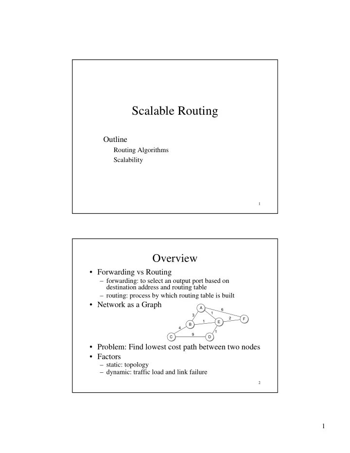
Scalable Routing Outline Routing Algorithms Scalability 1 Overview • Forwarding vs Routing – forwarding: to select an output port based on destination address and routing table – routing: process by which routing table is built • Network as a Graph A 6 1 3 2 F 1 E B 4 1 9 C D • Problem: Find lowest cost path between two nodes • Factors – static: topology – dynamic: traffic load and link failure 2 1

Distance Vector Algorithm • Each node maintains a set of triples – (Destination, Cost, NextHop) • Directly connected neighbors exchange updates – periodically (on the order of several seconds) – whenever table changes (called triggered update) • Each update is a list of pairs: – ( Destination, Cost) • Update local table if receive a “better” route – smaller cost – higher cost from the current NextHop (e.g. link failures) • Refresh existing routes; delete if they time out 3 Example B Destination Cost NextHop C A A 1 A D C 1 C D 2 C E E 2 A F G F 2 A G 3 A pp. 275 ~ 277, Tables 4.5 – 4.8 4 2

Routing Loops • Example 1: Fast Convergence – F detects that link to G has failed – F sets distance to G to infinity and sends update t o A – A sets distance to G to infinity since it uses F to reach G – A receives periodic update from C with 2-hop path to G – A sets distance to G to 3 and sends update to F – F decides it can reach G in 4 hops via A • Example 2: “Count to Infinity” due to the loop A-B-C – link from A to E fails – A advertises distance of infinity to E – B and C still advertise a distance of 2 to E periodically • NextHop is not in updates • Timing: sent before B, C receive (E, ∞ ) from A, received after (E, ∞ ). – B decides it can reach E in 3 hops; advertises this to A – A decides it can read E in 4 hops; advertises this to C – C decides that it can reach E in 5 hops… 5 Loop- Breaking Heuristics • Set infinity to 16 – Nodes can be reached beyond 16 links. – RIP (Routing Information Protocol) • Split horizon – For the triple (dest, cost, X), don’t include (dest, cost) in the update sent to X. – with poison reverse: for the triple (dest, cost, X), include (dest, ∞ ) in the update sent to X. – Solve loops involving two nodes (e.g. G x A ↔ B) – Cannot but solve loops of three or more nodes 6 3

Link State • Strategy – send to all nodes (not just neighbors) information about directly connected links (not entire routing table) • Link State Packet (LSP) – id of the node that created the LSP – cost of link to each directly connected neighbor – sequence number (SEQNO) – time-to-live (TTL) for this packet 7 Link State (cont) • Reliable flooding – store most recent (see seqno) LSP from each node – forward LSP to all nodes but one that sent it – generate new LSP periodically • increment SEQNO – start SEQNO at 0 when reboot – decrement TTL of each stored LSP • discard when TTL=0 8 4

Route Calculation • Dijkstra’s shortest path algorithm – See example on pp. 286 - 287 • Let – N denotes set of nodes in the graph – l ( i , j ) denotes non-negative cost (weight) for edge ( i , j ) – s denotes this node – C ( n ) denotes cost of the path from s to node n – M denotes the set of nodes incorporated so far M = { s } for each n in N - { s } C ( n ) = l ( s , n ) while ( N != M ) M = M union { w } such that C ( w ) is the minimum for all w in ( N - M ) for each n in ( N - M ) C ( n ) = MIN( C ( n ), C ( w ) + l ( w, n )) 9 Metrics • Assigning “1” to each link is inefficient – Satellite links have higher propagation delays. – Links have different capacities • OSPF uses 100Mbps / C – Links have dynamic traffic loads • New ARPANET metric – for each packet, record its arrival time ( AT ) and record departure time ( DT ) – when link-level ACK arrives, compute Delay = (DT - AT) + Transmit + Latency – link cost = average delay over some time period – if timeout (link-level ACK used), reset DT to departure time for retransmission • DT- AT captures not only queuing delay, but also the link reliability 10 5

Metrics (cont) • Problems: – under heavy load, DT – AT dominates the delay. Traffic moves back and forth between links – A 56 kbps looks too costly than a 9.6 kbps terrestrial link (due to the long delay), making its bandwidth underutilized. • Revised Metrics (p.293) 225 9.6-Kbps satellite link 140 9.6-Kbps terrestrial link 56-Kbps satellite link 56-Kbps terrestrial link 90 75 60 30 11 25% 50% 75% 100% Utilization DV vs. LS • LS is more stable and robust – With DV, incorrect computation can spread to entire network. • LS avoids loops better • LS converges faster than DV • LS reveals the complete topology. • DV requires less memory and CPU time – maintains neighbor states only – no Dijkstra’s algorithm – Since LS floods LSP to entire network, seqno and hence checksum are introduced to guarantee consistency 12 6

Internet Structure Today ! Large corporation networks can be connected to Backbone. ! Consumers can be connected to ISPs ! Many providers arrange to interconnect to each other at a single “peering” point. Large corporation “Consumer”ISP Peering point Backbone service provider Peering point “Consumer”ISP “Consumer”ISP Large corporation Small corporation 13 How to Make Routing Scale • Flat versus Hierarchical Addresses • Inefficient use of Hierarchical Address Space – class C with 2 hosts (2/255 = 0.78% efficient) – class B with 256 hosts (256/65535 = 0.39% efficient) • Still Too Many Networks – routing tables and route propagation protocols do not scale • Subnetting – divide a “large” network number (e.g. class B) into smaller network spaces for physical networks with small numbers (< 65535) of hosts. • Supernetting – aggregate “small” network numbers (e.g. class C) into a “larger” network number for a physical network with more than 255 hosts 14 7

Subnetting • Add another level to address/routing hierarchy: subnet • Subnet masks define variable partition of host part – For networks with small number of hosts. – Do not have to align with byte boundary • Subnets visible only within site – routing scalability Network number Host number Class B address 111111111111111111111111 00000000 Subnet mask (255.255.255.0) Network number Subnet ID Host ID 15 Subnetted address Subnet Example Subnet mask: 255.255.255.128 Subnet number: 128.96.34.0 128.96.34.15 128.96.34.1 R1 H1 Subnet mask: 255.255.255.128 128.96.34.130 Subnet number: 128.96.34.128 128.96.34.139 128.96.34.129 H3 R2 H2 128.96.33.1 Forwarding table at router R1 128.96.33.14 Subnet Number Subnet Mask Next Hop Subnet mask: 255.255.255.0 128.96.34.0 255.255.255.128 interface 0 Subnet number: 128.96.33.0 128.96.34.128 255.255.255.128 interface 1 128.96.33.0 255.255.255.0 R2 16 8

Forwarding Algorithm • External routers only see class B network number: 128.96 – One entry is kept for all hosts under 128.96 • Internal routers and hosts use subnet masks: – (SubnetNum, SubnetMask, NextHop) – Routers search for a match : dest IP & SubnetMask == SubnetNum ? (SubnetNum & SubnetMask == SubnetNum) – Sending hosts use the above to see whether the dest IP is in the local subnet (e.g H1 → H2). – Use a default router if nothing matches 17 Supernetting • Assign block of contiguous network numbers to nearby networks – Called CIDR: Classless Inter-Domain Routing • Use a bit mask (CIDR mask) to identify block size • All routers must understand CIDR addressing • Efficient address allocation and Scalable Routing • Used by BGP • Forwarding: longest prefix match based on PATRICIA tree 18 9

Example: 2 levels of Supernetting • Corporation Y: 11000000 00000100 0000 • Corporation X: – Class C numbers: 192.4.16, …… 192.4.32 → 11000000 00000100 0001 • …… • AS: 11000000 000001 Corporation X (11000000000001000001) Border gateway (advertises path to Regional network 11000000000001) Corporation Y (11000000000001000000) 19 Route Propagation • Know a smarter router – hosts know local default router – local routers know site routers – site routers know core router – core routers know everything • Autonomous System (AS) – corresponds to an administrative domain – examples: University, company, backbone network – assign each AS a 16-bit number • Two-level route propagation hierarchy – interior gateway protocol (each AS selects its own) – exterior gateway protocol (Internet-wide standard) 20 10