[PPT] - Resonant Tunneling in a Dissipative Environment: Quantum Critical PowerPoint Presentation

SLIDE 1

1. Quantum mechanics + dissipation: open system  
resonant tunneling in a dissipative electromagnetic environment 
dissipation + symmetry of coupling → competition → QPT  
2. Quantum phase transition (QPT)  
change in ground state upon varying a parameter  
exotic state of matter at the critical point 
non-equilibrium properties??

Harold Baranger, Duke University

Resonant Tunneling in a Dissipative Environment: Quantum Critical Behavior

SG SG Source Drain Gate

SLIDE 2

Quantum Mechanics + Environment Tunneling with dissipation:

environment as a collection of oscillators-- a “bosonic bath” 
spin-boson model: 2 states + bosonic environment

[Feynman & Vernon, 1963] [Leggett, Dorsey, Fisher, Garg & Zwerger, RMP 1987]

Spin-boson model: 2 states + bosonic environment

e

QM tunneling

QPT

Classical behavior (2 degenerate states) Environmental modes suppresses tunneling.

SLIDE 3

After tunneling event, spreading of charge inhibited by environment → Coulomb interaction leads to a charging energy → blocks (suppresses) tunneling of electron In Quantum Transport Expt?: “Environmental Coulomb Blockade”

e

G dI/dV ~ max (eV, k T)

known

EF

energy position

[Reviews: Devoret,Esteve,Urbina LesHouches 95, Ingold&Nazarov 92,   Flensberg PhysicaScripta 91]

SLIDE 4

After tunneling event, spreading of charge inhibited by environment → Coulomb interaction leads to a charging energy → blocks (suppresses) tunneling of electron In Quantum Transport Expt?: “Environmental Coulomb Blockade”

e

G dI/dV ~ max (eV, k T)

known

EF

energy position

charge localized → Coulomb barrier

top view 

f structure

SLIDE 5

After tunneling event, spreading of charge inhibited by environment → Coulomb interaction leads to a charging energy → blocks (suppresses) tunneling of electron In Quantum Transport Expt?: “Environmental Coulomb Blockade”

e

G dI/dV ~ max (eV, k T)

known

EF

energy position

charge localized → Coulomb barrier still tunneling under Coulomb barrier

top view 

f structure

SLIDE 6

After tunneling event, spreading of charge inhibited by environment → Coulomb interaction leads to a charging energy → blocks (suppresses) tunneling of electron In Quantum Transport Expt?: “Environmental Coulomb Blockade”

e

G dI/dV ~ max (eV, k T)

known

EF

energy position

charge localized → Coulomb barrier still tunneling under Coulomb barrier finally comes out

top view 

f structure

SLIDE 7

r ≡ e2 h Rleads (≈ 0.75 here) G ∝ V 2r G ≡ dI dV

⇣ I ∝ V 2r + 1⌘

In Quantum Transport Expt?: “Environmental Coulomb Blockade”

e

G dI/dV ~ max (eV, k T)

known

After tunneling event, spreading of charge inhibited by environment

→ Coulomb interaction leads to a charging energy → blocks (suppresses) tunneling of electron measured observable: (differential) conductance, with EF

energy position

[Reviews: Devoret,Esteve,Urbina LesHouches 95, Ingold&Nazarov 92,   Flensberg PhysicaScripta 91]

SLIDE 8

carbon nanotube q.dot
dirty metal leads →
B=6T ⇒ “spinless”

R ∼ h e2

Outline

1. Experiment
2. Theory of approach to quantum critical point
3. Model of quantum critical system/state
map to interacting 1D model-- a Luttinger liquid
power laws from scaling at strong and weak coupling
amazing consistency with experiment!
introduce Majorana fermion representation
QCP described by a decoupled zero-mode Majorana
indirect experimental signature of Majorana: linear T dependence

SLIDE 9

Experimental System: Carbon Nanotube Quantum Dot Gleb Finkelstein group: H. Mebrahtu, I. Borzenets, Y. Bomze, A. Smirnov, GF  

SG SG Source Drain B=6 T (spinless case)

0.3 0.4 0.5 0.6 '6 '4 '2 2 4 6 V S G (V ) V gate2(V )

0.0 0.5 1.0

2

Sample: tuning the coupling asymmetry by the side gate Gate

Conductance, in units of e2/h Short carbon nanotube (CNT)   quantum dot (300 nm) connected   to resistive leads via   tunable tunnel barriers.

SLIDE 10

T = 4ΓLΓR (∆✏)2 + (ΓL + ΓR)2 G = e2 h T

Resonant Tunneling Ignore environment for now:   Tunneling through a double barrier → ¡resonances (sharp)

ΓR

ΓL

Symmetric coupling + on resonance → ¡perfect ¡transmission Conductance is Transmission!   (Landauer viewpoint) Now connect the environment-- what happens? is T suppressed? can tune

∆✏, ΓL, ΓR

B=6 T (spinless case)

SLIDE 11

G ∼ ⇣ max{eV, kBT} ⌘2r r ≡ e2 h Rleads (≈ 0.3 here)

Preliminary: Environmental Coulomb Blockade

0.1 1 10 100 1 10

G(V,T)/G(0,T) eV/kT

0.1 1

10

3

10

2

10

1

T (K)

Y Z

G (e

2/h)

1.0
0.5

0.0 0.5 1.0 10

3

10

2

10

1

Z

G (e

2/h)

V (mV)

Y

d c

Conductance far away from resonance → ¡single barrier case with “zero bias  anomaly”

SLIDE 12

Conductance Resonance: Symmetric vs. Asymmetric Coupling

Asymmetric

!30 !20 !10 10 20 30 1E !3 0.01 0.1 1

((((((((T ((K ) (2.0 (0.75 (0.18 (0.05

G ((e

2/h)

ΔV gate(mV )

!30 !20 !10 10 20 30 1E !3 0.01 0.1 1

G )(e

2/h)

ΔV gate(mV )

))))))))T )(K ) )2.0 )0.75 )0.18 )0.05

Symmetric [Mebrahtu, et al., Nature 488, 61 (2012)]

B=6 T (spinless case)

Rexpt. = 0.75(h/e2)

SLIDE 13

Conductance Resonance: Height and Width Power Laws

Asymmetric Symmetric

Height: Width:

0.1 1 0.01 0.1 1

G $(e

2/h)

T emperature$(K )

symmetric asymmetric

0.1 1 1

F WH M$(meV ) T emperature$(K )

symmetric asymmetric

Summary:

1 special point— symmetric & on resonance—

with perfect transmission,

for all other parameters, conduction blocked, G −

→ 0 G − → 1

SLIDE 14

0.1 1 1E-3 0.01 0.1 1 1-G (e /h) Temperature (K)

Peak 1 Peak 2

T1.2

d c

1 10 100 0.01 0.1 1-G (e

2/h)

V (µV)

V1.1

200 -100

100 200 0.6 0.7 0.8 0.9 1.0

0.055 0.18 0.75 0.07 0.26 1.10 0.09 0.34 1.36 0.11 0.41 1.67 0.15 0.58 1.96

G (e

2/h)

V (µV)

T (K)

d c b a

G~1 : Unstable, Strong-Coupling Fixed Point

unusual cusp in conductance!
power law approach to full transparency
V power and T power agree (quasi-linear)

[Henok Mebrahtu, et al., Nature Physics 2013]

SLIDE 15

0.1 1 10 0.01 0.1 1

T (mK) 340 260 180 150 110 90 70 55

G (e2/h)

ΔVgate(mV)/Tr/(r+1)(K)

ΔV

3.5

gate

a b c d

From G~1 to G=0: Flow Toward Weak-Coupling Fixed Point Shape of conductance resonance: use Vgate to tune resonant level through the chemical potential Remember simple double  barrier result:

T = 4ΓLΓR (∆✏)2 + (ΓL + ΓR)2

[Henok Mebrahtu, et al., Nature Physics 2013]

SLIDE 16

0.1 1 10 0.01 0.1 1

T (mK) 340 260 180 150 110 90 70 55

G (e2/h)

ΔVgate(mV)/Tr/(r+1)(K)

ΔV

3.5

gate

a b c d

From G~1 to G=0: Flow Toward Weak-Coupling Fixed Point Shape of conductance resonance: use Vgate to tune resonant level through the chemical potential Remember simple double  barrier result:

T = 4ΓLΓR (∆✏)2 + (ΓL + ΓR)2

Here: power in tail is 3.5 not 2 !

[Henok Mebrahtu, et al., Nature Physics 2013]

SLIDE 17

0.1 1 10 0.01 0.1 1

T (mK) 340 260 180 150 110 90 70 55

G (e2/h)

ΔVgate(mV)/Tr/(r+1)(K)

ΔV

3.5

gate

a b c d

From G~1 to G=0: Flow Toward Weak-Coupling Fixed Point Shape of conductance resonance: use Vgate to tune resonant level through the chemical potential Remember simple double  barrier result:

T = 4ΓLΓR (∆✏)2 + (ΓL + ΓR)2

Here: power in tail is 3.5 not 2 !

r ≡ e2 h Rleads (≈ 0.65 here)

Scaling collapse of data at different T

[Henok Mebrahtu, et al., Nature Physics 2013]

SLIDE 18

G ∼ T 2r, with r ≡ Re/(h2/e) G ∼ T 2(1/g−1)

Tunneling with Dissipation ↔ Luttinger Liquid physics

𝜒, 𝑢 =

ℏ ∫

𝑒𝑢𝑉, 𝑢

−

ℏ 𝑊𝑢

𝜒 = (𝜒 + 𝜒)/2 𝜒 = (𝜒 − 𝜒)/2

𝜒 𝜒

𝐿

=

< 4𝑕 − 1

0 < 𝑠 + 𝑠𝐻 < 2

𝑊

= 𝑊

𝐿

=

< 4𝑕 − 1 4𝑕𝑔 − 1 > 0 2 < 𝑠 + 𝑠𝐻 < 3
𝑊

= 𝑊 ¡

Finkelstein’s ¡group ¡at ¡

‘s ¡ –

Dissipative T

𝐻~max ¡ (𝑊

¡, 𝑈)

𝑠 = 𝑆/(ℎ/𝑓)

𝐻~𝑈/

Safi ¡& ¡

𝑕 = 1/(1 + 𝑠)

≠ ¡V

Г Г 𝐻 → 𝑓/ℎ

Г ≠Г

𝐻~𝑈/

𝜒(𝑢) → 𝜒(𝑢, 𝑦)

𝜒 𝑢 → 𝜒 𝑢, 𝑦 𝝌 𝝌𝒅 𝐼 𝜚 𝜚 𝜒′ 𝜒′

𝐡𝐠

𝑔/𝑑 𝐽 = 𝛽𝐽 − (1 − 𝛽)𝐽 𝜒 𝜒

𝑽, 𝑱 = 𝟏 ¡ 𝑉 𝐽

𝝌′

𝐿1

𝒉𝒈 𝒉𝒅 = 𝟐𝒔𝑯 𝟐𝒔

𝑠/𝑠

¡ ¡

𝒓 𝒒 ∑ 𝒓𝒋

𝒋

= 𝟏 𝒒𝒋 ∗ 𝒒𝒌 = (−𝟐)𝒋𝒌 𝜚 𝜚

≠V

𝑗 𝑘

𝑠

𝑕 𝑠/𝑠

0 < 𝑠 + 𝑠 < 2, ¡

𝑊

= 𝑊

2 < 𝑠 + 𝑠𝐻 < 3

𝑊

= 𝑊

𝜒

𝜚

𝑆 = ℎ/𝑓

𝑟 = 1, 𝑞 = −1 𝑟 = 1, 𝑞 = 1 𝑟 = −1, 𝑞 = 1 𝑟 = −1, 𝑞 = −1

𝜚 = (𝜚+𝜚)/ 2 ¡ 𝜚 = (𝜚−𝜚)/ 2

𝜒, 𝑢 =

ℏ ∫

𝑒𝑢𝑉, 𝑢

−
ℏ 𝑊𝑢

𝜒 = (𝜒 + 𝜒)/2 𝜒 = (𝜒 − 𝜒)/2

𝜒 𝜒

𝐿

=

< 4𝑕 − 1

0 < 𝑠 + 𝑠𝐻 < 2

𝑊

= 𝑊

𝐿

=

< 4𝑕 − 1 4𝑕𝑔 − 1 > 0 2 < 𝑠 + 𝑠𝐻 < 3
𝑊

= 𝑊 ¡

Finkelstein’s ¡group ¡at ¡

‘s ¡ –

𝐻~max ¡

(𝑊

¡, 𝑈)

𝑠 = 𝑆/(ℎ/𝑓)

𝐻~𝑈/

Safi ¡& ¡

𝑕 = 1/(1 + 𝑠)

≠ ¡V

Г Г 𝐻 → 𝑓/ℎ

Г ≠Г

𝐻~𝑈/

𝜒(𝑢) → 𝜒(𝑢, 𝑦)

𝜒 𝑢 → 𝜒 𝑢, 𝑦 𝝌 𝝌𝒅 𝐼 𝜚 𝜚 𝜒′ 𝜒′

𝐡𝐠

𝑔/𝑑 𝐽 = 𝛽𝐽 − (1 − 𝛽)𝐽 𝜒 𝜒

𝑽, 𝑱 = 𝟏 ¡ 𝑉 𝐽

𝝌′

𝐿1

𝒉𝒈 𝒉𝒅 = 𝟐𝒔𝑯 𝟐𝒔

𝑠/𝑠

¡ ¡

𝒓 𝒒 ∑ 𝒓𝒋

𝒋

= 𝟏 𝒒𝒋 ∗ 𝒒𝒌 = (−𝟐)𝒋𝒌 𝜚 𝜚

≠V

𝑗 𝑘

𝑠

𝑕 𝑠/𝑠

0 < 𝑠 + 𝑠 < 2, ¡

𝑊

= 𝑊

2 < 𝑠 + 𝑠𝐻 < 3

𝑊

= 𝑊

𝜒

𝜚

𝑆 = ℎ/𝑓

𝑟 = 1, 𝑞 = −1 𝑟 = 1, 𝑞 = 1 𝑟 = −1, 𝑞 = 1 𝑟 = −1, 𝑞 = −1

𝜚 = (𝜚+𝜚)/ 2 ¡ 𝜚 = (𝜚−𝜚)/ 2

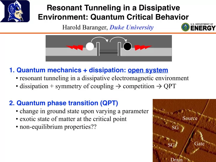
Single barrier (environmental Coulomb blockade):

g = 1 1 + r

𝜒, 𝑢 =

ℏ ∫

𝑒𝑢𝑉, 𝑢

−

ℏ 𝑊𝑢

𝜒 = (𝜒 + 𝜒)/2 𝜒 = (𝜒 − 𝜒)/2

𝜒 𝜒

𝐿

=

< 4𝑕 − 1

0 < 𝑠 + 𝑠𝐻 < 2

𝑊

= 𝑊

𝐿

=

< 4𝑕 − 1 4𝑕𝑔 − 1 > 0 2 < 𝑠 + 𝑠𝐻 < 3
𝑊

= 𝑊 ¡

Finkelstein’s ¡group ¡at ¡

‘s ¡ –

𝐻~max ¡

(𝑊

¡, 𝑈)

𝑠 = 𝑆/(ℎ/𝑓)

𝐻~𝑈/

Safi ¡& ¡Saleur, (2004)

𝑕 = 1/(1 + 𝑠)

≠ ¡V

Г Г 𝐻 → 𝑓/ℎ

Г ≠Г

𝐻~𝑈/

𝜒(𝑢) → 𝜒(𝑢, 𝑦)

𝜒 𝑢 → 𝜒 𝑢, 𝑦 𝝌 𝝌𝒅 𝐼 𝜚 𝜚 𝜒′ 𝜒′

𝐡𝐠

𝑔/𝑑 𝐽 = 𝛽𝐽 − (1 − 𝛽)𝐽 𝜒 𝜒

𝑽, 𝑱 = 𝟏 ¡ 𝑉 𝐽

𝝌′

𝐿1

𝒉𝒈 𝒉𝒅 = 𝟐𝒔𝑯 𝟐𝒔

𝑠/𝑠

¡ ¡

𝒓 𝒒 ∑ 𝒓𝒋

𝒋

= 𝟏 𝒒𝒋 ∗ 𝒒𝒌 = (−𝟐)𝒋𝒌 𝜚 𝜚

≠V

𝑗 𝑘

𝑠

𝑕 𝑠/𝑠

0 < 𝑠 + 𝑠 < 2, ¡

𝑊

= 𝑊

2 < 𝑠 + 𝑠𝐻 < 3

𝑊

= 𝑊

𝜒

𝜚

𝑆 = ℎ/𝑓

𝑟 = 1, 𝑞 = −1 𝑟 = 1, 𝑞 = 1 𝑟 = −1, 𝑞 = 1 𝑟 = −1, 𝑞 = −1

𝜚 = (𝜚+𝜚)/ 2 ¡ 𝜚 = (𝜚−𝜚)/ 2

mapping

[Safi & Saleur, PRL 04]

✓

Theoretical approach:

model in which tunneling event excites the environment
exploit formal correspondence to interacting 1D electrons
analyze resulting 1D quantum field theory
power laws come from scaling dimension of irrelevant and

relevant operators near the strong- and weak- coupling fixed points

[D. Liu, H. Zheng, S. Florens (Grenoble), HUB]

SLIDE 19

Need quantum description of electrical properties of the junctions S and D,  i.e. a quantum capacitor: introduce conjugate charge and   phase fluctuations on the junctions:

Model of Resonant Tunneling with Environment

ϕS,D(t) = e ~ Z t

1

dt0 δV (t0)

H =HDot + HLeads + HT + HT

Env

[ϕ, Q] = ie

H = Q2 2C + ϕ2 2L ✓~ e ◆2

HDot = ✏dd†d

HLeads = X

k

✏kc†

kSckS +

X

k

✏kc†

kDckD

After: Ingold & Nazarov review 1992, K. LeHur et al., C.-H. Chung et al., S. Florens et al.

SLIDE 20

ϕc ≡ (ϕS + ϕD)/2 ϕ ≡ ϕS − ϕD Model of Tunneling Junctions

electron destroyed in dot quasi-particle appears in metallic lead and   charge on junction shifts by 1e

HT = VS X

k

(c†

kSe−iϕSd + h.c.) + VD

X

k

(c†

kDe−iϕDd + h.c.)

eiϕQe−iϕ = Q − e

eiϕ

perator increments charge on capacitor by 1:

eiˆ

p

[remember action of on position] convenient to use sum and   difference variables: conjugate to total charge on dot

eiϕ moves charge around circuit

SLIDE 21

HT

Env = q2

2C + X

m

" q2

m

2Cm + ✓~ e ◆2 1 2Lm (ϕ − ϕm)2 #

Model of the Environment D eiϕ(t)e−iϕ(0)E ∝ 1 t2r

r ≡ Renviron. RQuant. Integrate out bath degrees of freedom to get correlation of phi: Couple phase to bath of LC oscillators:

choose oscillators such that the   impedance is ohmic (resistance R)

decay of quantum fluctuations of charge moving around the circuit  are controlled by the resistance

R

[Devoret, LesHouches 95]

SLIDE 22

Bosonic Description of Electrons in 1D, bosonize the fermionic leads

cS,D(x) = 1 √ 2πa FS,D exp[iφS,D(x)]

Leads: free fermions → ¡chiral ¡fermions ¡→ ¡bosonize [Wait! why 1D?? a local quantum system couples to only 1 continuous degree of freedom: mathematically: can always tri-diagonalize H starting from given state] X X X X X X dot

φS(x) φD(x)

and are standard chiral bosonic fields: density fluctuations of the electrons in the leads

SLIDE 23

φS,D = (φ0

c ± φ0 f)/

√ 2

HT = X

S,D VS,DFS,D √ 2πa

e−i 1

√ 2 [φ0 c(x=0)±φ0 f (x=0)]e−i(ϕc±ϕ/2)d + h.c.

φf ≡ √gf

φ0

f + 1 √ 2ϕ

H = HDot + vF

4π Z ∞

−∞

dx h (∂xφc)2 + (∂xφf)2i

+ X

S,D

h

VS,DFS,D p 2πa

e

⌥i

1

p2gf φf (x=0)ei 1

√ 2 φc(x=0)d + h.c.

i

Mapping to Luttinger Liquid

Emulate Luttinger liquid physics using E&M environment Goal: combine these lead fields with the environmental phase Combine so that fields in leads remain free; boundary op. changes:

gf ≡ 1 1 + r ≤ 1 with r ≡ Re RQ

SLIDE 24

Analysis of the Effective 1D Interacting Model To solve: draw on enormous literature on LL physics

[resonant level: Kane&Fisher 92, Eggert&Affleck 92, Furusaki 98,   Nazarov&Glazman 03, Komnik&Gogolin 03, Meden, et al. 05, Goldstein&Berkovits 10, ...]

side gate

“healed chain” fixed point:  competition between the two leads prevents the level from being absorbed into either one 

integrate out all quadratic degrees of freedom
perform perturbative RG-- “Coulomb gas RG”
at strong-coupling fixed point, analyze likely dominant operators

resulting   RG flow   diagram

(on resonance):

G~1

SLIDE 25

cos

2√πφx=0
∂xφx=0

cos

2√πφx=0
G ∼ T 2r

1 − G ∼ T

r r+1

1 − G ∼ T

2 r+1

Operators Controlling the Flow

Most important effect on transmission:   2kF scattering (back scattering) from the barriers in bosonized form, this corresponds to the operator This operator is irrelevant-- controls flow into the QCP along symmetric line If the coefficient of this leading operator is exactly 0  (ie. on-resonance and with symmetric barriers), then the next-to-leading operator is corresponds to 2kF scattering off the Friedel oscillation in the density This operator is relevant-- causes flow to weak coupling

→ for low conductance,

near unitary conductance,

→ near unitary conductance,

SLIDE 26

gate

2

0.1 1 10 1E-3 0.01 0.1 1 G (e

2/h)

ΔVgate(mV)/(T, V/a)r/(r+1)(K)

Vbias (µV) 70 ΔV-3.5

gate

c d

0.1 1 1

F WH M$(meV ) T emperature$(K )

Gpeak vs T (asym.)

2 r + 1 = 1.14 2(r + 1) = 3.5 r r + 1 = 0.43 2r = 1.5

Comparing Exponents to Experiment Tail of peak vs Vgate Gwidth vs T (sym.) Gpeak vs T or V (sym.) 1.1 or 1.2 3.4 0.45

0.1 1 0.01 0.1 1

G $(e

2/h)

T emperature$(K )

0.1 1 1E-3 0.01 0.1 1 1-G (e2/h) Temperature (K)

Peak 1 Peak 2

T1.2

d c

used to extract  r=0.75

✓✓✓

SLIDE 27

HT ∼ X

S,D

h

VS,DFS,D p 2πa

e

⌥i

1

p2gf φf (x=0)ei 1

√ 2 φc(x=0)d + h.c.

i ∼ e

−i

1

√2gf φf (x=0)⇥

VS d + VD d†⇤ + e

+i

1

√2gf φf (x=0)⇥

VD d + VS d†⇤ Strong Coupling Critical State: Majorana Fermion

What is special about the model Hamiltonian at the critical point? reorganize, drop inessential factors If , only the combination appears!

VS = VD d + d†

(current around the loop involves both   destruction and creation of the dot electron)

SLIDE 28

Majorana Hamiltonian for the QCP

First, unitary transform eliminates field from tunneling term:

φc

U = exp ⇥ i(d†d − 1/2)φc(0)/ √ 2 ⇤

H = HDot + HLeads + h

VSFS √ 2πae −i

1

√2gf φf (x=0)d + VDFD √ 2πa e +i

1

√2gf φf (x=0)d + h.c.

i

−π~vF (d†d − 1/2)∂xφc(x = 0)

, generating a density-density term [as in Komnik & Gogolin PRL 03; like Emery & Kivelson for 2 channel Kondo]

ψ†

f ≡ FS √ 2πae−iφf (x=0)

Second, refermionize for g=1/2 (ie. r=1): competition between leads is like competition between channels in 2CK-- leads to Majorana representation in same way

SLIDE 29

HMajorana = HLeads+ (VS − VD) ⇥ †

f(0) − f(0)

⇤ a + i(VS + VD) ⇥ †

f(0) + f(0)

⇤ b + 2i✏dab − 2i⇡~vF †

c(0) c(0)ab

S = 1

2 log 2

S = 1

2 log(1 + r)

Majorana Hamiltonian for the QCP

one Majorana hybridizes with the leads
the other is uncoupled (when symmetric and on resonance)

[much as in describing the two-channel Kondo problem]

d† = a − ib

Write the state in the quantum dot as two Majorana’s:

an independent Majorana zero mode

˜ g ∝ (1 − r)

In experiment, r is not quite 1 : interacting leads with

[Wong &  Affleck]

If neglect contact interaction: Majorana resonant level  → ¡non-interacting model, so dependence on T and V is quadratic 

SLIDE 30

HMajorana = HLeads+ (VS − VD) ⇥ †

f(0) − f(0)

⇤ a + i(VS + VD) ⇥ †

f(0) + f(0)

⇤ b + 2i✏dab − 2i⇡~vF †

c(0) c(0)ab

S = 1

2 log 2

S = 1

2 log(1 + r)

Majorana Hamiltonian for the QCP

one Majorana hybridizes with the leads
the other is uncoupled (when symmetric and on resonance)

[much as in describing the two-channel Kondo problem]

d† = a − ib

Write the state in the quantum dot as two Majorana’s:

an independent Majorana zero mode

˜ g ∝ (1 − r)

In experiment, r is not quite 1 : interacting leads with

[Wong &  Affleck]

If neglect contact interaction: Majorana resonant level  → ¡non-interacting model, so dependence on T and V is quadratic 

SLIDE 31

−2iπ~vF ψ†

c(0)ψc(0)ab

Gb(t) ≡ ⌦ b+(0)b(t) ↵ ∝ 1/t

Gψc(x=0)(t) ∝ 1/t Ga(t) = ⌦ a+(0)a(t) ↵ ∝ 1

Σb(t) ∝ v2

F Ga(t)G2 ψc(t) ∝ 1/t2

1 − G ∝ T 1

ˆ I = V ⇥ ψf(0) − ψ†

f(0)

⇤ b Majorana Hamiltonian: Linear Conductance from Interactions

If neglect contact interaction: Majorana resonant level  → ¡non-interacting model, so dependence on T and V is quadratic  But in system studied, the interaction is large, ~EF   Nevertheless, try perturbation theory: physical current in transformed basis:

ψf unaffected by interaction  

→ ¡correction to G=1 comes from self-energy of b ¡Majorana!

linear dependence on T or V is signature of Majorana fermion

If r not 1, ~near linear dependence...

→ →

by Fourier transform

[H. Zheng, S. Florens, HB, PRB 2014]

SLIDE 32

0.1 1 1E-3 0.01 0.1 1 1-G (e /h) Temperature (K)

Peak 1 Peak 2

T1.2

d c

1 10 100 0.01 0.1 1-G (e

2/h)

V (µV)

V1.1

200 -100

100 200 0.6 0.7 0.8 0.9 1.0

0.055 0.18 0.75 0.07 0.26 1.10 0.09 0.34 1.36 0.11 0.41 1.67 0.15 0.58 1.96

G (e

2/h)

V (µV)

T (K)

d c b a

G~1 : Unstable, Strong-Coupling Fixed Point

unusual cusp in conductance!
power law approach to full transparency
V power and T power agree (quasi-linear)

[Henok Mebrahtu, et al., Nature Physics 2013]

non-quadratic dependence is signature of Majorana zero mode

SLIDE 33

Æ Resonant tunneling in a

dissipative environment  

dissipation + symmetry of coupling → competition → QPT

Æ 1. Experiment: Beautiful data accessing both  strong- and weak- coupling fixed points Æ 2. Theory: mapping to interacting 1D model-- emulation of LL  uncoupled Majorana state → ~linear dependence of 1-G Majorana Quantum Critical Behavior for   Resonant Level + Dissipative Environment

CONCLUSIONS

D. Liu, H. Zheng, S. Florens, HUB 
H. Mebrahtu, I. Borzenets,Y. Bomze,  
A. Smirnov, G. Finkelstein

[Mebrahtu, et al., Nature 488, 61 (2012), Nature Physics (2013)]