Reinforcement Learning CS 4100: Artificial Intelligence - PDF document

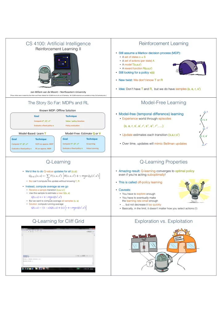
Reinforcement Learning CS 4100: Artificial Intelligence Reinforcement Learning II • Still assume a Marko kov decision process (MDP): • A se set o of st states s s Î S • A se set o of a actions ( s (per st state) A • A mo model T( T(s,a s,a,s ,s’) ’) • A re reward rd functio ion R( R(s,a s,a,s ,s’) ’) • Still looki king for a policy p (s) s) • Ne New twist st: We d We don’t kn know T or or R • Id Idea: Don’t have T and R , but we do have sa samples (s (s, a, r, s’) Jan-Willem van de Meent – Northeastern University [These slides were created by Dan Klein and Pieter Abbeel for CS188 Intro to AI at UC Berkeley. All CS188 materials are available at http://ai.berkeley.edu.] The Story So Far: MDPs and RL Model-Free Learning Known MDP: Offline Solution s • Mod Model el-fr free ( (te temporal d diffe fference) l learning a Goal Technique • Exp xperience world through episo sodes s, a Compute V*, Q*, p * Value / policy iteration r Evaluate a fixed policy p Policy evaluation (s, s, a, r, s’ s’, a’, r’, s’ s’’, a’’, r’’, …) …) s’ a’ Model-Based: Learn T Model-Free: Estimate Q or V • Up Update estimates each transition (s, s,a,r,s’) ’) s’, a’ Goal Technique Goal Technique • Over time, updates will mi mimi mic c Bel ellman man up updat ates es Compute V*, Q*, p * Compute V*, Q*, p * Q Learning s’’ VI/PI on approx. MDP Evaluate a fixed policy p Value Learning Evaluate a fixed policy p PE on approx. MDP Q-Learning Q-Learning Properties • Amazi • We’d like zing resu sult: Q-le learnin ing converges to optimal policy y ke to do Q-va value updates s for all (s, s,a): even if you’re acting su suboptimally ! • Bu But can’t compute this update without knowing T, T, R • This s is s called of off-policy y learning • Inst stead, compute ave verage as s we go • Cave veats: s: • Receive ve a sa sample transition (s, s,a,r,s’) ’) • Use this sample to estimate a a new new Q(s, s, a) • You have to exp xplore enough • You have to eventually make • But we want to compute average all sa the learning rate sm small enough samples s (s, a , a) • So Solution: compute running average • … but not decrease it too quickl kly • Basically, in the limit, it doesn’t matter how you select actions (!) Q-Learning for Cliff Grid Exploration vs. Exploitation

How to Explore? Q-learning – Epsilon-Greedy – Crawler • Seve veral sc schemes s for forcing exp xploration • Simplest st: random actions ( e -gr greedy dy ) • Every time step, flip a coin • With (small) probability e , act act rand andom omly • With (large) probability 1- e , act act on on cur current ent pol olicy cy • Problems s with random actions? s? • You do eventually explore the space, but keep thrashing around once learning is done solution: lower e over time • One so • Another so solution: exploration functions [Demo: Q-learning – manual exploration – bridge grid (L11D2)] [Demo: Q-learning – epsilon-greedy -- crawler (L11D3)] Exploration Functions Q-learning – Exploration Function – Crawler • When to exp xplore? • Random actions: s: explore a fixed amount • Be Better idea: explore areas whose badness is not (yet) established, eventually stop exploring • Exp xploration function • Takes a va value est stimate u and a vi visi sit count n , and returns an optimist stic ut utility , e.g. Regular Q-Update: Modified Q-Update: • No s” back to states that lead to unknown states! Note: this propagates the “bonus” [Demo: exploration – Q-learning – crawler – exploration function (L11D4)] Regret Approximate Q-Learning • To l To lear earn n the the op opti timal al p pol olicy cy, yo you need need to to make ke mist stake kes s along the way! y! • Re Regret measu sures s the cost st of yo your mist stake kes: s: • Difference between your (expected) rewards, including youthful suboptimality, and (expected) rewards for an agent that optimally balances exploration and exploitation. • Minimizi zing regret is a stronger condition than acting optimally y – also measures whether you have le learned optim imally lly • Exa xample: random exploration and exploration functions both end up optimal, but random exploration has higher regret Generalizing Across States Q-Learning Pacman – Tiny World • Basi sic Q-Lear Learni ning ng ke keeps s a table of all q-va values • In realist stic si situations, s, we cannot possi ssibly y learn about eve le very y si single st state! • Too many states to visit them all in training • Too many states to hold the q-tables in memory • Inst stead, we want to generalize ze: • Learn about some small number of training states from experience • Generalize that experience to new, similar situations • This is a fundamental idea in machine learning, and we’ll see it over and over again [demo – RL pacman]

Q-Learning Pacman – Tiny – Silent Train Q-Learning Pacman – Tricky Example: Pacman Feature-Based Representations • Ide Idea: : desc scribe a st state s usi sing a ve vector Let’s say we discover In naïve q-learning, Or even this one! of hand of hand-cr craf afted ed fe featu tures (properties) s) through experience we know nothing that this state is bad: about this state: • Features states to real numbers s are functions from st s (often 0/1) that capture properties of the state • Exa xample features: s: • Distance to closest ghost • Distance to closest dot • Number of ghosts • 1 / (dist to dot) 2 • Is Pacman in a tunnel? (0/1) • …… etc. • Is it the exact state on this slide? • Can also describe a q-st state (s, s, a) with features (e.g. action moves closer to food) [Demo: Q-learning – pacman – tiny – watch all (L11D5)],[Demo: Q-learning – pacman – tiny – silent train (L11D6)], [Demo: Q-learning – pacman – tricky – watch all (L11D7)] Approximate Q-Learning Linear Value Functions • Usi sing a a feature represe sentation , we can define a q fu q functi tion (or va value function ) for any st state s s using a small number of weights w : • Q-le learnin ing wit with lin linear Q-fu functi tions: Exact Q’s • Adva vantage: our experience is summed up in a few powerful numbers Approximate Q’s • Intuitive ve interpretation: • Disa sadva vantage: states that share features may have very different values! • Adjust we weig ights ts of active ve features • If something unexpectedly bad happens, blame the features that were ‘on’. • Formal just stification: online least squares Example: Q-Pacman Approximate Q-Learning -- Pacman [Demo: approximate Q- learning pacman (L11D10)]

Linear Approximation: Regression* Q-Learning and Least Squares 40 26 24 20 22 20 30 40 20 0 30 0 20 20 10 10 0 0 Prediction: Prediction: Optimization: Least Squares* Minimizing Error* Imagine we had only one point x , with features f( f(x) , target value y , and weights w : Error or “residual” Observation Prediction Approximate q-up update explained: 0 “target y” “prediction f(x)” 0 20 Overfitting: Why Limiting Capacity Can Help* Policy Search 30 25 20 Degree 15 polynomial 15 10 5 0 -5 -10 -15 0 2 4 6 8 10 12 14 16 18 20 Policy Search Policy Search • Pr • Simplest Probl blem: o : ofte ften th the fe featu ture-base sed policies s that work k well (win games, s, maxi ximize ze st policy y se search: utilities) s) aren’t the ones s that have ve the best st V V / Q / Q approxi ximation • Start with an initial linear va value function or Q-fu functi tion • E.g. your va value functions s from pr project 2 were probably horrible • Nu Nudge each feature we weig ight up and down wn and estimates of future rewards, but they st still produced good decisi sions see if your policy is better than before • Q-learning’s s priority: y: get Q-va values s close (modeling) • Action se selection priority: y: get ordering of Q-va values s right (prediction) • Problems: s: • We’ll see this distinction between modeling and prediction again later in the course • How do we tell the policy got better? • Need to run many sample episodes! • So Soluti tion: : learn po policies that maximize rewards, not the va values s that predict them • If there are a lot of features, this can be impractical • Policy y se search: start with an ok solution (e.g. Q-le learnin ing ) then fi fine-tu tune • Better methods exploit lookahead structure, by hill climbing on feature weights sample wisely, change multiple parameters…

RL: Helicopter Flight RL: Learning Locomotion [Andrew Ng] [Video: HELICOPTER] [Video: GAE] [Schulman, Moritz, Levine, Jordan, Abbeel, ICLR 2016] RL: Learning Soccer RL: Learning Manipulation [Bansal et al, 2017] [Levine*, Finn*, Darrell, Abbeel, JMLR 2016] RL: NASA SUPERball RL: In-Hand Manipulation Pieter Abbeel -- UC Berkeley | Gradescope | [Geng*, Zhang*, Bruce*, Caluwaerts, Vespignani, Sunspiral, Abbeel, Levine, ICRA 2017] Pieter Abbeel -- UC Berkeley | Gradescope | Covariant.AI Covariant.AI OpenAI: Dactyl Conclusion • We’r We’re e done one wit with h Pa Part I t I: Se : Search a and Pl d Planning! g! • We’ve ve se seen how AI methods s can so solve ve problems s in: • Se Search • Const straint Satisf sfaction Problems • Ga Games • Marko kov v Decisi sion Problems • Re Reinforcement Learning • Next xt up up Pa Part II t II: Uncertainty y and Learning! Trained with domain randomization [OpenAI]