Reinforcement Learning CS 188: Artificial Intelligence - - PowerPoint PPT Presentation

CS 188: Artificial Intelligence

Reinforcement Learning

Instructors: Pieter Abbeel and Dan Klein University of California, Berkeley

[These slides were created by Dan Klein and Pieter Abbeel for CS188 Intro to AI at UC Berkeley. All CS188 materials are available at http://ai.berkeley.edu.]

Reinforcement Learning Reinforcement Learning

§ Basic idea:

§ Receive feedback in the form of rewards § Agent’s utility is defined by the reward function § Must (learn to) act so as to maximize expected rewards § All learning is based on observed samples of outcomes! Environment

Agent

Actions: a State: s Reward: r

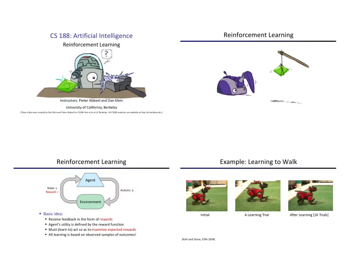
Example: Learning to Walk

Initial A Learning Trial After Learning [1K Trials]

[Kohl and Stone, ICRA 2004]

Example: Learning to Walk

Initial

[Video: AIBO WALK – initial] [Kohl and Stone, ICRA 2004]

Example: Learning to Walk

Training

[Video: AIBO WALK – training] [Kohl and Stone, ICRA 2004]

Example: Learning to Walk

Finished

[Video: AIBO WALK – finished] [Kohl and Stone, ICRA 2004]

Example: Sidewinding

[Andrew Ng] [Video: SNAKE – climbStep+sidewinding]

Example: Toddler Robot

[Tedrake, Zhang and Seung, 2005] [Video: TODDLER – 40s]

The Crawler!

[Demo: Crawler Bot (L10D1)] [You, in Project 3]

Video of Demo Crawler Bot Reinforcement Learning

§ Still assume a Markov decision process (MDP):

§ A set of states s Î S § A set of actions (per state) A § A model T(s,a,s’) § A reward function R(s,a,s’)

§ Still looking for a policy p(s) § New twist: don’t know T or R

§ I.e. we don’t know which states are good or what the actions do § Must actually try out actions and states to learn

Offline (MDPs) vs. Online (RL)

Offline Solution Online Learning

Model-Based Learning Model-Based Learning

§ Model-Based Idea:

§ Learn an approximate model based on experiences § Solve for values as if the learned model were correct

§ Step 1: Learn empirical MDP model

§ Count outcomes s’ for each s, a § Normalize to give an estimate of § Discover each when we experience (s, a, s’)

§ Step 2: Solve the learned MDP

§ For example, use value iteration, as before

Example: Model-Based Learning

Input Policy p

Assume: g = 1

Observed Episodes (Training) Learned Model A

B C

D

E

B, east, C, -1 C, east, D, -1 D, exit, x, +10 B, east, C, -1 C, east, D, -1 D, exit, x, +10 E, north, C, -1 C, east, A, -1 A, exit, x, -10

Episode 1 Episode 2 Episode 3 Episode 4

E, north, C, -1 C, east, D, -1 D, exit, x, +10

T(s,a,s’).

T(B, east, C) = 1.00 T(C, east, D) = 0.75 T(C, east, A) = 0.25 …

R(s,a,s’).

R(B, east, C) = -1 R(C, east, D) = -1 R(D, exit, x) = +10 …

Example: Expected Age

Goal: Compute expected age of cs188 students

Unknown P(A): “Model Based” Unknown P(A): “Model Free”

Without P(A), instead collect samples [a1, a2, … aN]

Known P(A) Why does this work? Because samples appear with the right frequencies. Why does this work? Because eventually you learn the right model.

Model-Free Learning Passive Reinforcement Learning Passive Reinforcement Learning

§ Simplified task: policy evaluation

§ Input: a fixed policy p(s) § You don’t know the transitions T(s,a,s’) § You don’t know the rewards R(s,a,s’) § Goal: learn the state values

§ In this case:

§ Learner is “along for the ride” § No choice about what actions to take § Just execute the policy and learn from experience § This is NOT offline planning! You actually take actions in the world.

Direct Evaluation

§ Goal: Compute values for each state under p § Idea: Average together observed sample values

§ Act according to p § Every time you visit a state, write down what the sum of discounted rewards turned out to be § Average those samples

§ This is called direct evaluation

Example: Direct Evaluation

Input Policy p

Assume: g = 1

Observed Episodes (Training) Output Values A

B C

D

E

B, east, C, -1 C, east, D, -1 D, exit, x, +10 B, east, C, -1 C, east, D, -1 D, exit, x, +10 E, north, C, -1 C, east, A, -1 A, exit, x, -10

Episode 1 Episode 2 Episode 3 Episode 4

E, north, C, -1 C, east, D, -1 D, exit, x, +10

A

B C

D

E

+8 +4 +10

• 10
• 2

Problems with Direct Evaluation

§ What’s good about direct evaluation?

§ It’s easy to understand § It doesn’t require any knowledge of T, R § It eventually computes the correct average values, using just sample transitions

§ What bad about it?

§ It wastes information about state connections § Each state must be learned separately § So, it takes a long time to learn

Output Values A

B C

D

E

+8 +4 +10

• 10
• 2

If B and E both go to C under this policy, how can their values be different?

Why Not Use Policy Evaluation?

§ Simplified Bellman updates calculate V for a fixed policy:

§ Each round, replace V with a one-step-look-ahead layer over V § This approach fully exploited the connections between the states § Unfortunately, we need T and R to do it!

§ Key question: how can we do this update to V without knowing T and R?

§ In other words, how to we take a weighted average without knowing the weights? p(s) s s, p(s) s, p(s),s’ s’

Sample-Based Policy Evaluation?

§ We want to improve our estimate of V by computing these averages: § Idea: Take samples of outcomes s’ (by doing the action!) and average

p(s) s s, p(s) s1' s2' s3' s, p(s),s’ s'

Almost! But we can’t rewind time to get sample after sample from state s.

Temporal Difference Learning Temporal Difference Learning

§ Big idea: learn from every experience!

§ Update V(s) each time we experience a transition (s, a, s’, r) § Likely outcomes s’ will contribute updates more often

§ Temporal difference learning of values

§ Policy still fixed, still doing evaluation! § Move values toward value of whatever successor occurs: running average

p(s) s s, p(s) s’ Sample of V(s): Update to V(s): Same update:

Exponential Moving Average

§ Exponential moving average

§ The running interpolation update: § Makes recent samples more important: § Forgets about the past (distant past values were wrong anyway)

§ Decreasing learning rate (alpha) can give converging averages

Example: Temporal Difference Learning

Assume: g = 1, α = 1/2

Observed Transitions

B, east, C, -2 8

• 1

8

• 1

3

8 C, east, D, -2

A

B C

D

E States

Problems with TD Value Learning

§ TD value leaning is a model-free way to do policy evaluation, mimicking Bellman updates with running sample averages § However, if we want to turn values into a (new) policy, we’re sunk: § Idea: learn Q-values, not values § Makes action selection model-free too!

a s s, a s,a,s’ s’

Active Reinforcement Learning Active Reinforcement Learning

§ Full reinforcement learning: optimal policies (like value iteration)

§ You don’t know the transitions T(s,a,s’) § You don’t know the rewards R(s,a,s’) § You choose the actions now § Goal: learn the optimal policy / values

§ In this case:

§ Learner makes choices! § Fundamental tradeoff: exploration vs. exploitation § This is NOT offline planning! You actually take actions in the world and find out what happens…

Detour: Q-Value Iteration

§ Value iteration: find successive (depth-limited) values

§ Start with V0(s) = 0, which we know is right § Given Vk, calculate the depth k+1 values for all states:

§ But Q-values are more useful, so compute them instead

§ Start with Q0(s,a) = 0, which we know is right § Given Qk, calculate the depth k+1 q-values for all q-states:

Q-Learning

§ Q-Learning: sample-based Q-value iteration § Learn Q(s,a) values as you go

§ Receive a sample (s,a,s’,r) § Consider your old estimate: § Consider your new sample estimate: § Incorporate the new estimate into a running average:

[Demo: Q-learning – gridworld (L10D2)] [Demo: Q-learning – crawler (L10D3)]

Video of Demo Q-Learning -- Gridworld Video of Demo Q-Learning -- Crawler

Q-Learning Properties

§ Amazing result: Q-learning converges to optimal policy -- even if you’re acting suboptimally! § This is called off-policy learning § Caveats:

§ You have to explore enough § You have to eventually make the learning rate small enough § … but not decrease it too quickly § Basically, in the limit, it doesn’t matter how you select actions (!)