Reinforcement Learning CS 4100: Artificial Intelligence - PowerPoint PPT Presentation

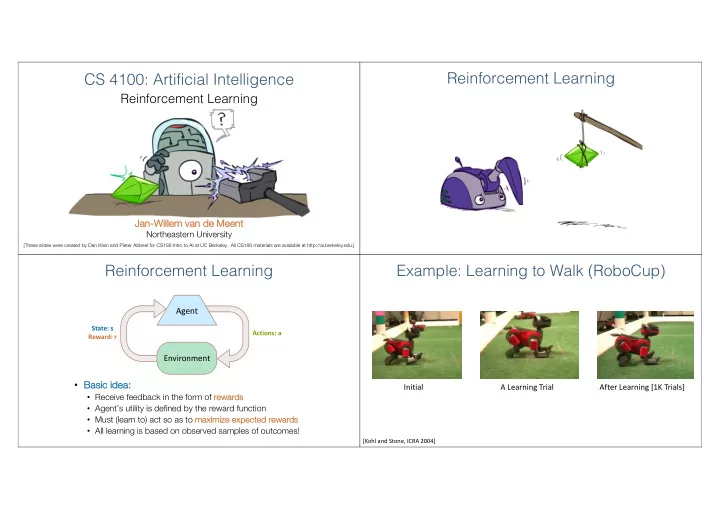
Reinforcement Learning CS 4100: Artificial Intelligence Reinforcement Learning Ja Jan-Wi Willem van de Meent Northeastern University [These slides were created by Dan Klein and Pieter Abbeel for CS188 Intro to AI at UC Berkeley. All CS188 materials are available at http://ai.berkeley.edu.] Reinforcement Learning Example: Learning to Walk (RoboCup) Agent State: s Actions: a Reward: r Environment • Ba Basic ic id idea: Initial A Learning Trial After Learning [1K Trials] • Receive feedback in the form of re reward rds • Agent’s utility is defined by the reward function • Must (learn to) act so as to ma maximi mize ze expected rewards • All learning is based on observed samples of outcomes! [Kohl and Stone, ICRA 2004]

Example: Learning to Walk Example: Learning to Walk Initial (lab-trained) Training [Kohl and Stone, ICRA 2004] [Kohl and Stone, ICRA 2004] [Video: AIBO WALK – initial] [Video: AIBO WALK – training] Example: Learning to Walk Example: Sidewinding Finished [Kohl and Stone, ICRA 2004] [Video: AIBO WALK – finished] [Andrew Ng] [Video: SNAKE – climbStep+sidewinding]

Example: Toddler Robot The Crawler! [Tedrake, Zhang and Seung, 2005] [Video: TODDLER – 40s] [Demo: Crawler Bot (L10D1)] [You, in Project 3] Reinforcement Learning Video of Demo Crawler Bot • Still assume a Marko kov decision process (MDP): • A se set o of st states s s Î S • A se set o of a actions ( s (per st state) A • A mo model T( T(s,a s,a,s ,s’) ’) • A re reward rd functio ion R( R(s,a s,a,s ,s’) ’) king for a policy p (s) • Still looki s) • Ne New twist st: We d We don’t ’t kn know T or or R • I.e. we don’t know which states are good or what the actions do • Must actually try out actions and states to learn

Offline (MDPs) vs. Online (RL) Model-Based Learning Offline Solution Online Learning Example: Model-Based Learning Model-Based Learning • Mo Input Policy p Observed Episodes (Training) Learned Model Model-Base sed Idea: • Learn an approxi ximate model based on experiences Episode 1 Episode 2 T(s,a,s’). • Solve ve for va values as if the learned model were correct T(B, east, C) = 1.00 B, east, C, -1 B, east, C, -1 A • St Step p 1: Learn empir piric ical l MDP DP mode del T(C, east, D) = 0.75 C, east, D, -1 C, east, D, -1 • Co T(C, east, A) = 0.25 Count outcomes s’ s’ for each s , a D, exit, x, +10 D, exit, x, +10 … • Normalize B C ze to give an estimate of D • Disc scove ver each when we experience (s, s, a, s’ s’) Episode 3 Episode 4 E • Step 2: Solve ve the learned MDP E, north, C, -1 E, north, C, -1 R(B, east, C) = -1 • For example, use va R(C, east, D) = -1 value iteration , as before C, east, D, -1 C, east, A, -1 R(D, exit, x) = +10 Assume: g = 1 D, exit, x, +10 A, exit, x, -10 …

Example: Expected Age Model-Free Learning Goal: Compute expected age of CS4100 students Known P(A) Without P(a), instead collect samples [a 1 , a 2 , … a N ] Unknown P(A): “Model Based” Unknown P(A): “Model Free” Why does this Why does this work? Because work? Because eventually you samples appear learn the right with the right model. frequencies. Passive Reinforcement Learning Passive Reinforcement Learning • Simplified task: sk: policy y eva valuation t: a fixed policy p (s) • In Inpu put: s) • You don’t know the transitions T( T(s, s,a,s’) ’) • You don’t know the rewards R( R(s, s,a,s’) ’) • Go Goal: learn the state values V(s) s) • In this s case se: • Learner is “along for the ride” • No choice about what actions to take • Just execute the policy and learn from experience • This is NOT offline planning! You actually take actions in the world.

Example: Direct Evaluation Direct Evaluation Input Policy p Observed Episodes (Training) Output Values state under p • Go Goal: Compute va values for each st Episode 1 Episode 2 • Id Idea: Average over observed sample values -10 B, east, C, -1 B, east, C, -1 A Act according to p • Ac A C, east, D, -1 C, east, D, -1 • Every time you visit a state, write down what D, exit, x, +10 D, exit, x, +10 +8 +4 +10 B C D B C the sum of discounted rewards turned out to be D • Ave verage those samples Episode 3 Episode 4 -2 E E E, north, C, -1 E, north, C, -1 • This is called direct eva valuation C, east, D, -1 C, east, A, -1 Assume: g = 1 D, exit, x, +10 A, exit, x, -10 Problems with Direct Evaluation Why Not Use Policy Evaluation? Output Values s • Wh What at’s ’s g good ab about d direct ect ev eval aluat ation? • Si Simplifi fied Bellman updates calculate V fo for a fi fixed policy: • It’s easy to understand • Ea Each round , replace V with a on one-st step-lo look-ah ahead ead p (s) -10 • It doesn’t require any knowledge of T, T, R A s, p (s) • It eventually computes the correct average +8 +4 +10 values, using just sample transitions B C s, p (s),s’ D s’ -2 • This approach fully exploited the connections between the states • Wh What at’s ’s b bad ad ab about i it? E • Un Unfort rtunately ly , we need T and R to do it! • It wastes information about state connections If B and E both go to C • Each state must be learned separately under this policy, how can • Key Key ques estion: how can can we e do this updat ate e to V without kn knowing T an and R? • So, it takes a long time to learn their values be different? • In other words, how to we take a weighted average without knowing the weights?

Sample-Based Policy Evaluation? Temporal Difference Learning • We w We wan ant t to im improve ou our r estima mate of of V by by compu omputing g av aver erag ages es: • Id Idea: Take samples of ou outcome omes s’ s’ (by doing the action!) and average s p (s) s, p (s) s, p (s),s’ s 1 ' s' s 2 ' s 3 ' Almost! But we can’t rewind time to get sample after sample from state s. Temporal Difference Learning Exponential Moving Average • Bi Big idea: learn n from every experienc nce! s • Exp xponential movi ving ave verage • Up Update V( V(s) each time we experience a transition (s (s, a, s’, r) p (s) • Runni unning ng in interpola latio ion update: • Like kely outcomes s’ s’ will contribute updates more often s, p (s) • Makes recent sa samples s more important: • Te Tempor oral diffe fference learning g of of values • Po Policy is still fi fixed , still doing evaluation! s’ • Mo Move values toward value of whatever successor occurs: ru running a avera rage Samp Sa mple of V( V(s): • Forgets s about the past st (distant past values were wrong anyway) Update to V( Up V(s): • Decreasi ing rate α can give converging averages sing le learnin Same Sa me update:

Example: Temporal Difference Learning Problems with TD Value Learning St States Ob Observed Transitions • TD TD value leaning g is a mode model-fr free way to do pol policy evaluation on , mimicking Bellman updates with running sample averages B, east, C, -2 C, east, D, -2 • However, if we want to turn va values into a (new) pol policy , we’re sunk: A 0 0 0 s B C D 0 0 -1 0 -1 3 8 8 8 a E 0 0 0 s, a • Id Idea: learn Q-va values , not va values s,a,s’ Assume: g = 1 , α = 1/2 • Makes action selection model-free too! s’ Active Reinforcement Learning Active Reinforcement Learning • Ful Full rei reinf nforcement orcement learni earning ng: optimal policies s (like value iteration) • You don’t know the transitions T( T(s, s,a,s’) ’) • You don’t know the rewards R( R(s, s,a,s’) ’) • You choose the actions now • Go Goal: l : learn th the o opti ptimal policy y / va values • In this s case se: • Learner makes choices! • Fund Fundam ament ental al trad adeof eoff: exploration vs. exploitation • This s is s NOT offline planning! You actually take actions in the world and find out what happens…

Detour: Q-Value Iteration Q-Learning • Q-Learni ng: sample-based Q-va Learning value iteration tion: find successive (depth-limited) va • Va Value ite terati values • St Start with V 0 (s) = = 0 , which we know is right • Giv Given V k , calculate the depth k+1 k+1 values for all states: • Learn Learn Q( Q(s, s,a) ) va values s as s yo you go • Receive a sample (s, s,a,s’ s’,r) • Consider your old estimate: • But But Q-va values ar are e more e usefu eful, so compute them instead • Consider your new sample estimate: • St Start with Q 0 (s, s,a) = = 0 , which we know is right • Giv Given Q k , calculate the depth k+1 k+1 q-values for all q-states: • Incorporate the new estimate into running average: [Demo: Q-learning – gridworld (L10D2)] [Demo: Q-learning – crawler (L10D3)] Q-Learning -- Gridworld Q-Learning -- Crawler

Q-Learning Properties • Amazi ing converges to optimal policy zing resu sult: Q-le learnin y even if you’re acting suboptimally! • This s is s called of off-policy y learning • Cave veats: s: • You have to explore enough • You have to eventually make the learning rate small enough • … but not decrease it too quickly • Basically, in the limit, it doesn’t matter how you select actions (!)