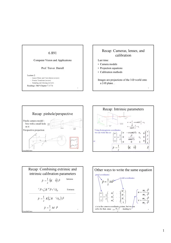
Recap: Cameras, lenses, and 6.891 calibration Computer Vision and - PDF document

Recap: Cameras, lenses, and 6.891 calibration Computer Vision and Applications Last time: • Camera models Prof. Trevor. Darrell • Projection equations • Calibration methods Lecture 2: – Linear Filters and Convolution (review) Images are projections of the 3-D world onto – Fourier Transform (review) – Sampling and Aliasing (review) a 2-D plane… Readings: F&P Chapter 7.1-7.6 1 2 Recap: Intrinsic parameters Recap: pinhole/perspective Pinole camera model - x y � � cot( � ) u � � Г u 0 box with a small hole z z � y in it: v � Г v 0 sin( � ) z Perspective projection: Using homogenous coordinates, � � x � � � � � cot( � ) we can write this as: u � � � � 0 u 0 � � � � � � 1 � y � � � 0 0 � v � v � � 0 � � � x sin( � ) z z � � � x ' f ' � � � 1 � 0 � or: � � � z � � 0 0 1 � � � 1 � � y � � y ' f ' 1 � � � � � z � � p � K 0 P 3 4 z Forsyth&Ponce Recap: Combining extrinsic and Other ways to write the same equation intrinsic calibration parameters pixel coordinates world coordinates 1 � � Intrinsic � 1 � � � P p � K 0 � p M P � z z C C W C � P R P O Extrinsic � Г m P � W W � � W 1 T x u � � � � � � � u � . m . . 1 � � � � m P � W � � 1 3 T y � � � 1 � v � . m . . � � � � � C C 2 � � P p K R O m P � z W � � � � � W W T z 2 � � v 1 . m . . � z � � � � � � � 3 1 m P � � � 3 1 � z is in the camera coordinate system, but we can � � p � Μ P m P � solve for that, since , leading to: 3 5 6 1 z � z Forsyth&Ponce 1

� m P Recap: � 1 u � � m � P 3 � Camera calibration m P Today � 2 v � � m P � 3 Stack all these measurements of i=1…n points Review of early visual processing � ( m u m ) P 0 � � � – Linear Filters and Convolution 1 i 3 i � ( m v m ) P 0 � � � – Fourier Transform 2 i 3 i into a big matrix: – Sampling and Aliasing T T T � � � � � P 0 u P 0 1 1 1 � � You should have been exposed to this material in � � � � T T T m � � � 0 P v P 1 0 previous courses; this lecture is just a (quick) � � � � 1 1 1 � � � � � � � � � review. m � � 2 � � � � T T T 0 � � � Administrivia: P 0 u P m � n n n � � � � � 3 � � � � – sign-up sheet 0 T T T � 0 P v P � � � � n n n – introductions 7 8 What is image filtering? Linear functions • Simplest: linear filtering. • Modify the pixels in an image based on – Replace each pixel by a linear combination of some function of a local neighborhood of its neighbors. the pixels. • The prescription for the linear combination is called the “convolution kernel”. 10 5 3 Some function 10 5 3 0 0 0 4 5 1 7 4 5 1 0 0.5 0 7 1 1 7 1 1 7 0 1 0.5 Local image data Modified image data 9 Local image data kernel Modified image data 10 Convolution Linear filtering (warm-up slide) coefficient f [ m , n ] � I � g � � I [ m � k , n � l ] g [ k , l ] 1.0 k l , ? 0 Pixel offset original 11 12 2

Linear filtering (warm-up slide) Linear filtering coefficient coefficient 1.0 1.0 ? 0 Pixel offset 0 Pixel offset original original Filtered (no change) 13 14 shift Linear filtering coefficient coefficient 1.0 0.3 ? 0 0 Pixel offset Pixel offset original original shifted 15 16 Blur examples Blurring coefficient 8 2.4 impulse 0.3 coefficient 0 filtered original Pixel offset 0.3 0 Pixel offset original Blurred (filter applied in both dimensions). 17 18 3

Blur examples Smoothing reduces noise coefficient 8 2.4 • Generally expect pixels to • Implies that smoothing impulse “be like” their neighbours suppresses noise, for 0.3 appropriate noise models – surfaces turn slowly – relatively few reflectance • Scale 0 filtered original Pixel offset changes – the parameter in the • Generally expect noise symmetric Gaussian coefficient processes to be – as this parameter goes up, 8 8 more pixels are involved in independent from pixel to the average pixel edge 4 4 0.3 – and the image gets more blurred – and noise is more 0 filtered original Pixel offset effectively suppressed 19 20 Linear filtering (warm-up slide) The effects of smoothing 2.0 Each row shows smoothing with gaussians of different 1.0 width; each column shows different realisations of ? an image of gaussian noise. 0 0 original 21 22 Linear filtering (no change) Linear filtering 2.0 2.0 1.0 0.33 ? 0 0 0 0 Filtered original original (no change) 23 24 4

Linear filtering (remember blurring) 2.0 coefficient 0.33 0.3 ? 0 0 0 Pixel offset original original Blurred (filter applied in both dimensions). 25 26 Sharpening Sharpening example 2.0 1.7 11.2 coefficient 8 8 0.33 0 0 -0.25 -0.3 Sharpened original Sharpened original original (differences are accentuated; constant areas are left untouched). 27 28 Sharpening Gradients and edges • Points of sharp change • General strategy in an image are – linear filters to estimate interesting: image gradient – change in reflectance – mark points where – change in object gradient magnitude is – change in illumination particularly large wrt – noise neighbours (ideally, • Sometimes called curves of such points). before after edge points 29 30 5

Smoothing and Differentiation • Issue: noise – smooth before differentiation – two convolutions to smooth, then differentiate? – actually, no - we can use a derivative of Gaussian filter 1 pixel • because differentiation is convolution, and convolution is 3 pixels 7 pixels associative The scale of the smoothing filter affects derivative estimates, and also the semantics of the edges recovered. 31 32 Oriented filters Linear image transformations Gabor filters (Gaussian modulated • In analyzing images, it’s often useful to harmonics) at different make a change of basis. scales and spatial frequencies transformed image � � Vectorized image F U f � Top row shows anti-symmetric (or odd) filters, bottom row the symmetric (or even) filters. Fourier transform, or Wavelet transform, or Steerable pyramid transform 33 34 An example of such a transform: the Fourier transform Self-inverting transforms discrete domain Forward transform � km ln � M � 1 N � 1 � Г � i � � Same basis functions are used for the inverse transform � M N � F [ m , n ] �� f [ k , l ] e � � � � � � 1 k 0 l 0 f U F � � Г U F � Inverse transform � km ln � � � M 1 N 1 Г Г i � � 1 � � M N � f [ k , l ] �� F [ m , n ] e � MN k � 0 l � 0 U transpose and complex conjugate 35 36 6

Here u and v To get some sense of what are larger than basis elements look like, we in the previous plot a basis element --- or slide. rather, its real part --- as a function of x,y for some fixed u, v. We get a function that is constant when (ux+vy) is constant. The magnitude of the vector (u, v) gives a frequency, and its direction gives an orientation. The function is a sinusoid with this frequency along the direction, and constant perpendicular to the direction. 37 38 And larger still... Phase and Magnitude • Fourier transform of a real • Curious fact function is complex – all natural images have about the same magnitude – difficult to plot, visualize transform – instead, we can think of the – hence, phase seems to phase and magnitude of the matter, but magnitude transform largely doesn’t • Phase is the phase of the • Demonstration complex transform – Take two pictures, swap the • Magnitude is the phase transforms, compute magnitude of the complex the inverse - what does the transform result look like? 39 40 This is the magnitude transform of the cheetah pic 41 42 7

This is the phase transform of the cheetah pic 43 44 This is the This is the magnitude phase transform transform of the zebra of the zebra pic pic 45 46 Reconstruction with zebra Reconstruction phase, cheetah with cheetah magnitude phase, zebra magnitude 47 48 8

Example image synthesis with 2 fourier basis. • 16 images 49 50 6 18 51 52 50 82 53 54 9

136 282 55 56 538 1088 57 58 2094 4052. 4052 59 60 10

8056. 15366 61 62 28743 49190. 63 64 65536. Fourier transform magnitude 65 66 11