SLIDE 1 Thin Lenses Thick Lenses
2 2 2
1 1 1
i i i i T
L
f s s x x f y s M y s dx f M dx x = + = ≡ = − ≡ = −
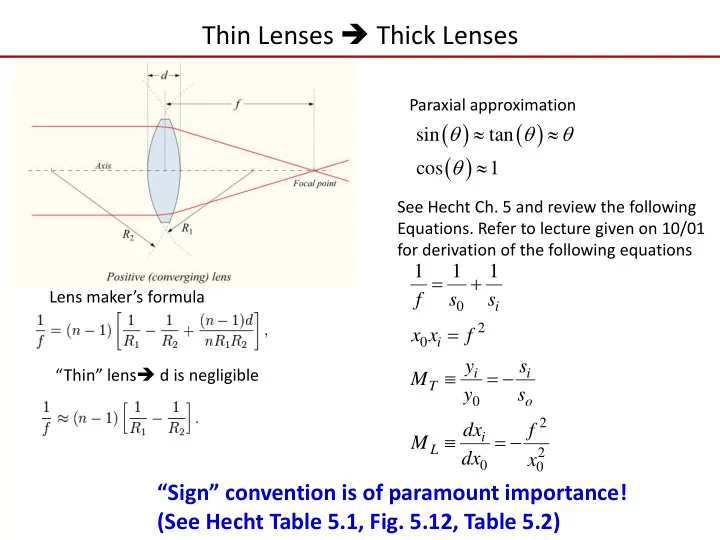
Paraxial approximation Lens maker’s formula “Thin” lens d is negligible
( ) ( ) ( )
sin tan cos 1 θ θ θ θ ≈ ≈ ≈
See Hecht Ch. 5 and review the following
- Equations. Refer to lecture given on 10/01
for derivation of the following equations
“Sign” convention is of paramount importance! (See Hecht Table 5.1, Fig. 5.12, Table 5.2)
SLIDE 2
Recall : Real and Virtual Images
See also Hecht Table 5.3
SLIDE 3
Numerical Aperture
Paraxial approximation
( ) ( )
sin tan / 2 1 2 / # D NA f f θ θ θ ≈ ≈ → = =
We will learn that the spatial resolution limit due to diffraction ≈ 1.22×f λ /D=0.61×λ/NA [Rayleigh Criterion].
SLIDE 4 When Paraxial Approximation Fails: Ray Tracing + Diffraction
- Databases of common lenses and elements
- Simulate aberrations and ray scatter diagrams for
various points along the field of the system (PSF, point spread function)
- Standard optical designs (e.g. achromatic doublet)
- Permit optimization of design parameters (e.g.
curvature of a particular surface or distance between two surfaces) vs designated functional requirements (e.g. field curvature and astigmatism coefficients)
- Also account for diffraction by calculating the at
different points along the field modulation transfer function (MTF) [Fourier Optics]
SLIDE 5 Aberrations
Refractive index n is dispersive!
( )
n ω
(monochromatic) Deteriorate the image:
- Spherical aberration
- Coma
- Astigmatism
Deform the image:
- Field curvature
- Distortion
Departures from the idealized conditions of Gaussian Optics (e.g. paraxial regimes).
SLIDE 6
Chromatic Aberration
Hecht 6.3.2
SLIDE 7 Chromatic Aberration
Melles Griot “Fundamental Optics” Solutions:
- 1. Combine lenses (achromatic doublets)
- 2. Use mirrors
SLIDE 8
Spherical Aberration
Solution I: Aspheric Mirrors or Lenses
SLIDE 9
Hubble Telescope
It was probably the most precisely figured mirror ever made, with variations from the prescribed curve of only 10 nanometers, it was too flat at the edges by about 2.2 microns. Source: wikipedia
SLIDE 10
Lens Shape
Solution II: Chose a proper shape of a singlet lens for a given image-object distance. ( ) ( )
1 2 2 1
R R q R R + = −
For a given desired focal length, there is freedom to choose one of the radii for a singlet. The spherical aberration and coma depend on the particular choice, so these aberrations can be minimized by the designed form.
SLIDE 11
Lens Selection Guide
http://www.newport.com/Lens-Selection-Guide/140908/1033/catalog.aspx#
SLIDE 12
Astigmatism
SLIDE 13
Coma and Deformation