Random Access Networks Random Access networks are characterised by - - PDF document

Chapter 3

Random Access Networks

Random Access networks are characterised by the absence of a channel- controlled access mechanism. To some extent, a station is free to broadcast its packets on the network at a time determined by the station itself, with never any certainty that another station is not simultaneously attempting a transmission.

3.1 The ALOHA Procedure

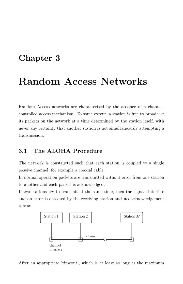
The network is constructed such that each station is coupled to a single passive channel, for example a coaxial cable. In normal operation packets are transmitted without error from one station to another and each packet is acknowledged. If two stations try to transmit at the same time, then the signals interfere and an error is detected by the receiving station and no acknowledgement is sent.

Station1 Station2 Station M

channel interface channel

After an appropriate ’timeout’, which is at least as long as the maximum

EE414 Notes - The ALOHA Procedure 25 two-way propagation time of the cable, the original transmitting stations conclude that a collision has occurred and schedule retransmission of the packets at later times. To avoid repeated collisions of packets, the retransmission times are usually chosen at random by the stations involved.

3.1.1 Throughput Analysis of ALOHA

• Let P seconds be the transmission time for a packet (propagation time

+ transmission time).

• Let

Pr[k arrivals in t seconds] = (Λt)k k! e−Λt be the Poisson distribution describing all transmissions over the chan- nel where Λ = arrival rate in Pkts/Sec . This expression assumes an infinite population of infrequent users.

• Let S be the average number of successful transmissions per packet

transmission time P.

• Let G be the average number of attempted packet transmissions per

packet transmission time P.

startofpacket time time 2P P

startofpacket transmission conclusionofpacket transmission

P P

Vunerableintervalforstartofpacketsthatcolide withreferencestationpacket

startofpacket

Packettransmissiontime

Figure 3.1: Vulnerable Period for ALOHA

EE414 Notes - The ALOHA Procedure 26 Figure 9.1 (top) shows some packet being transmitted. The lower diagram shows the positioning of other packets that just avoid colliding with the

• riginal packet. The ’vunerable’ period can be seen to be of length 2P.

A relationship between S and G is: S = G Pr[Good Transmission] The probability of a good transmission is the probability of no additional transmissions in the vulnerable period of length 2P about the transmission

• f the original packet.

Pr[0 arrivals in an interval of length 2P] = e−2G as Λ = G/P therefore S = Ge−2G

EE414 Notes - The ALOHA Procedure 27

Offeredtraffic, G Throughput, S 0.10 0.15 0.20 1/2e 0.10 ( , ) G'S' 0.5

Figure 3.2: S vs G for ALOHA A plot of this relationship is shown in Figure 9.2. Note that S has a maxi- mum value of

1 2e ≈ 0.184 for G = 0.5.

In producing this graph it is assumed that the system is in statistical equi- librium for the average quantities S and G. This is not always the case. Consider the point (G′, S′). If G′ increases slightly due to statistical fluctu- ations in the offered load, the throughput S decreases. This further increases the backlog and hence load G. Therefore the operating point moves further to the right. This continues and the system becomes saturated. Thus the system is in an unstable operating region for G > 0.5.

EE414 Notes - The ALOHA Procedure 28

3.1.2 Average Packet Transfer Delay of ALOHA

The average number of attempts per successfully transmitted packet is given by: G/S = e2G Therefore, the average number of unsuccessful attempts per successfully transmitted packet is given by: G/S − 1 = e2G − 1 If a collision occurs, the station reschedules the colliding packet for some randomly chosen later time. The average backoff delay is denoted by B. The average transfer delay is given by: T = P + (e2G − 1)(P + B) The value of B depends on the backoff strategy. The lower bound on the delay is at B = 0: Tmin = Pe2G

EE414 Notes - Slotted ALOHA 29

3.2 Slotted ALOHA

The Slotted ALOHA procedure segments the time into slots of a fixed length P. Every packet transmitted must fit into one of these slots. A packet arriving to be transmitted at any given station must be delayed until the beginning of the next slot. Slotted ALOHA requires additional overhead to provide the synchronisation. The station can be in either of two states:

• Transmitting
• Backed-off

To avoid repeated collisions, collided packets are rescheduled at later times chosen independently and at random.

EE414 Notes - Slotted ALOHA 30

Packet Ready? Delayto Beginningof Slot Transmit Wait2-Way PropDelay Quantisedto Slots Positive Ack? Exit Compute Random BackoffInteger ( ) k Delay kP Backoff Algorithm No Yes No Yes

Figure 3.3: Flow Diagram for Slotted ALOHA Procedure

EE414 Notes - Slotted ALOHA 31

3.2.1 Throughput Analysis of Slotted ALOHA

An expression for S in terms of G is required. This will be derived for an infinite population and a finite population of stations.

• Throughput S
• Offered Load G (per interval P)

As in the Pure ALOHA derivation, both new arrivals and retransmissions due to collisions, form a Poisson process with mean arrival rate Λ pack- ets/sec. (Note that Λ = G/P).

time P

Vunerableperiodfor slotted ALOHA

P

ReferencePacket

Figure 3.4: Vulnerable Period for slotted ALOHA The vulnerable period for Slotted ALOHA is reduced from 2P to P seconds. Throughput and offered load are related by the same equation as before: S = G Pr[Successful Transmission] Thus we have for Slotted ALOHA: Pr[no arrival in an interval of length P] = e−ΛP = e− G

P P ⇒

S = Ge−G Compare this with the Pure Aloha case: S = Ge−2G The maximum throughput for Slotted ALOHA is 1

e ≈ 0.368 and the maxi-

mum occurs for G = 1.

EE414 Notes - Slotted ALOHA 32

Offeredtraffic, G Throughput, S 0.10 0.30 0.40 1/e 0.01 0.5 1.0 0.1 0.05 0.20

ALOHA Slotted ALOHA

Figure 3.5: S vs G for ALOHA and Slotted ALOHA Finite Population Case In the above we have assumed the number of users is infinite. Here we will revise the model for a finite population and determine under what conditions the infinite population model gives a reasonable approximation. Consider a network with M independent stations. The input from each station is modelled as a sequence of independent Bernoulli Trials. Let Si be the probability of station i successfully transmitting a packet in any slot. 1 − Si is the probability of not successfully transmitting a packet. Let Gi and 1 − Gi be the probabilities for attempting and not attempting transmissions respectively. The probability that station j has a successful transmission is the probability that station j is the only station to attempt a transmission in a particular

• slot. Therefore:

Sj = Gj

M

• i=1

i=j

(1 − Gi) Assuming all stations share the load equally then S = MSj and G = MGj, therefore: S = G(1 − G/M)M−1

EE414 Notes - Slotted ALOHA 33 Note that: lim

n→∞

• 1 + X

n n = eX as M → ∞ ∴ as M → ∞ S = Ge−G (as before) For M stations the maximum throughput Smax is calculated by differenti- ating and equating to zero: 0 =

• 1 − G

M

• − G

M − 1 M

• which results in G = 1 (as for the infinite case)

Smax =

• 1 − 1

M M−1 This approaches the infinite result (0.368) as M → ∞ and is reasonably close for M ≥ 20. Thus it is reasonable to assume an infinite population in the analysis when we are modelling any reasonably large network.

3.2.2 Analysis of Slotted ALOHA Taking Backoff into Ac- count

The analyses given earlier account for retransmissions only by increasing the

• ffered traffic. These analyses assumed that both new and collided packets

come from the same process and did not account for the delays that collided packets experience. The following analysis accounts for newly arrived and retransmitted packets as separate variables to give greater accuracy in the analysis. Here we wish to derive:

• 1. Average Transfer Delay - Throughput relation
• 2. Throughput - Offered Load expression which is more accurate

The following assumptions and definitions are made:

• The population of users is infinite.
• New arrivals to the network come from a Poisson process with mean

arrival rate S packets/slot or Λ packets/sec where S = ΛP (where P = ¯ X/R).

EE414 Notes - Slotted ALOHA 34

• The total arrival process of packets to the network, including new

arrivals and retransmissions is Poisson with mean arrival rate G pack- ets/slot.

• Each station has at most one packet ready for transmission, including

any previously collided packets.

• End-to-end propagation delay for the complete bus is τ seconds.
• Transmitting station learns whether or not transmission is successful

after a time rounded to r slots. (Where r the smallest integer > 2τ

P ).

• The processing time of the receiver is negligible in comparison to the

propagation delay.

P rP

Initial transmission

kP

Transmittingstation awareofcollision Initiationof retransmission

Backoff Time

Figure 3.6: Timing Diagram for Slotted ALOHA To determine the backoff time, an integer k is selected at random from the set {0, 1, 2, . . . , K − 1} with each integer equally likely. Retransmission takes place P + rP + kP seconds later. The average backoff time is given by: kP = 1 K

K−1

• k=0

kP = K − 1 2

• P

An average backoff cycle (defined as the total time required to transmit a packet, determine that it has collided, and wait the backoff time) thus requires: P + rP + (K − 1)P 2 = rP + (K + 1)P 2 seconds The total transfer delay of a packet has four components:

• 1. The waiting time after arrival until the beginning of the next slot

EE414 Notes - Slotted ALOHA 35

• 2. The delay due to retransmission
• 3. The packet transmission time
• 4. The propagation delay

The average of each of these quantities must be determined and summed. Item 1: Arrivals can occur at any stage in the previous packet transmission time P. All times are equally likely ∴ average waiting time = P

2 seconds.

Item 3: Transmission time is constant at P seconds Item 2: Average retransmission delay was determined as: rP + (K + 1)(P/2) seconds for each cycle Let H = average number of retransmission cycles. Then H[rP + (K + 1)(P/2)] seconds is the average time required for all retransmission. Item 4: If stations are uniformly distributed along the cable, then the aver- age delay is the delay over 1

3 the cable length = τ/3.

These four components can be added to give the total average delay: T = P + P/2 + τ/3 + H

• rP + K + 1

2 P

• H must now be determined in terms of S, G and K.

First define qn and qt: qn Probability of a successful transmission given that the transmission is with a new packet qt Probability of a successful transmission given that the transmission is a retransmission The probability, pi, that a given packet requires exactly i retransmissions can now be expressed in terms of qn and qt as: pi = (1 − qn)(1 − qt)i−1qt i ≥ 1

EE414 Notes - Slotted ALOHA 36 The average number of retransmissions is determined from pi by the equa- tion: H =

∞

• i=1

i pi Thus, using the previous two equations: H = 1 − qn qt The average total delay is: T = P + P/2 + τ/3 + 1 − qn qt rP + K + 1 2

• P
• qn and qt are related to S, G and K by (not derived here):

qt =

• e−G/K − e−G

1 − e−G e−G/K + G

K e−GK−1

e−S (∗) qn =

• e−G/K + G

K e−GK

e−S (∗) G/S = the average number of times a packet must be transmitted until success. 1 + H = G/S (∗) Using the expression for H gives an equation relating the offered load and throughput: S = G

• qt

1 + qt − qn

• This is a more accurate expression than previously calculated. However, as

K → ∞: qn → e−G qt → e−G and S = Ge−G as before. The above three equations (*) can be solved to eliminate qn and qt. An analytic solution is not appropriate and the result is more easily obtained numerically.

EE414 Notes - Slotted ALOHA 37 The three equations (*) can be rearranged into the form: S B(G, K) + SeS = A(G, K) where A(G, K) = GeSqt and B(G, K) = eSqt − eSqn Note that these expressions depend only on G and K. A graph can be formed (Figure 9.7) by setting values for G and K and then solving for S.

Offeredtraffic, G Throughput, S 0.10 0.30 0.40 0.01 1.0 0.1 0.20

K=2 K=5 K=20 K=

8

Figure 3.7: S vs G for Slotted ALOHA for Various Values of K

3.2.3 Nomalised Delay

It is useful to obtain an expression for normalised delay by dividing the expression for T by P: T = 3

2P + τ/3 +

1 − qn qt rP + K + 1 2 P

• ˆ

T = 3

2 + a/3 +

1 − qn qt

• [r + K/2 + 1

2]

where a = τ/P is the normalised end-to-end propagation delay.

EE414 Notes - Slotted ALOHA 38

3.2.4 Average Number in Backlog

Because backoff delay = queueing delay we can use Little’s Law to determine the average number ¯ N in the backlog. ¯ N = (S/P)H

• rP +

K + 1 2

• P
• where

H = 1 − qn qt

• ¯

N = SH[r + 1/2 + K/2]