SLIDE 1
R preliminaries for Survival Course.
Page | 1
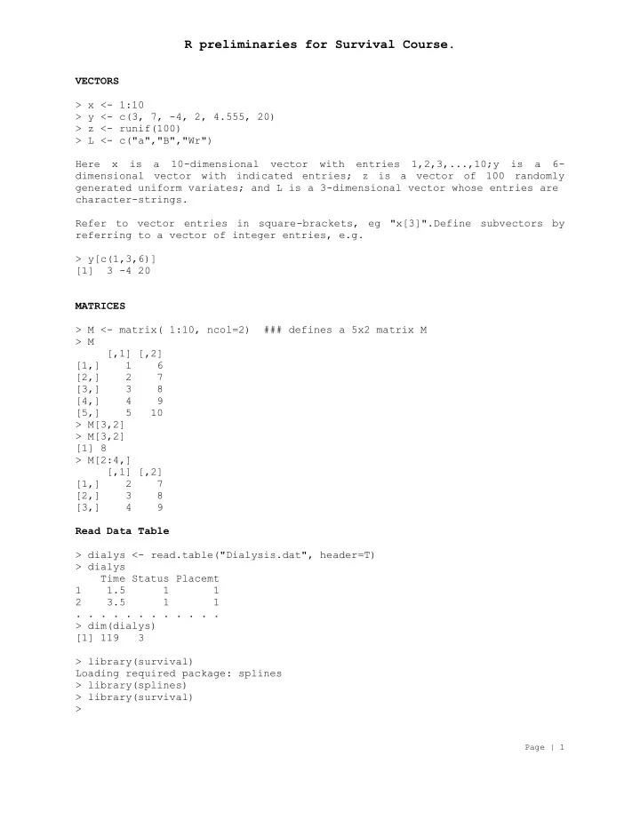
VECTORS > x <- 1:10 > y <- c(3, 7, -4, 2, 4.555, 20) > z <- runif(100) > L <- c("a","B","Wr") Here x is a 10-dimensional vector with entries 1,2,3,...,10;y is a 6- dimensional vector with indicated entries; z is a vector of 100 randomly generated uniform variates; and L is a 3-dimensional vector whose entries are character-strings. Refer to vector entries in square-brackets, eg "x[3]".Define subvectors by referring to a vector of integer entries, e.g. > y[c(1,3,6)] [1] 3 -4 20 MATRICES > M <- matrix( 1:10, ncol=2) ### defines a 5x2 matrix M > M [,1] [,2] [1,] 1 6 [2,] 2 7 [3,] 3 8 [4,] 4 9 [5,] 5 10 > M[3,2] > M[3,2] [1] 8 > M[2:4,] [,1] [,2] [1,] 2 7 [2,] 3 8 [3,] 4 9 Read Data Table > dialys <- read.table("Dialysis.dat", header=T) > dialys Time Status Placemt 1 1.5 1 1 2 3.5 1 1 . . . . . . . . . . . . > dim(dialys) [1] 119 3 > library(survival) Loading required package: splines > library(splines) > library(survival) >
SLIDE 2
R preliminaries for Survival Course.
Page | 2
The trial was conducted by matching pairs of patients at a given hospital by remission status (complete or partial) and randomizing within the pair to either a 6-MP or placebo maintenance therapy. Patients were followed until their leukemia returned (relapse)or until the end of the study (in months). The data is reported in Table 1.1. 1st column is ID of patient pair, (one randomized to 6MP, one to placebo 2nd column is initial Remission Type (1=partial, 2=complete) 3rd and 4th columns time to relapse resp. for Placebo and 6MP patients 5th column is status = indicator of relapse for 6MP patient > Leuk <- read.table("Leukem.txt")[,2:5] > names(Leuk) = c("RemTyp","Pcb.tim","6MP.tim","6MP.Rlps") >Leuk RemTyp Pcb.tim 6MP.tim 6MP.Rlps 1 1 1 10 1 2 2 22 7 1 3 2 3 32 0 . . . . . . . . . . . . . . . . . . > dim(Leuk) [1] 21 4
SLIDE 3
R preliminaries for Survival Course.
Page | 3
Exponential distribution: > t <- seq(from = 1, to = 100, by = 1) > lambda = 0.25 > ht <- lambda > Ht <- lambda * t > St <- exp(-lambda * t) > par(mfrow = c(2,3), pty = "s") > plot(t, rep(ht, times = length(t)),ylim = c(0, 1), lwd = 2, type = "s", xlab = "Time", ylab = "h(t)") > plot(t, Ht,ylim = c(0, 25),lwd = 2,type = "s", xlab = "Time", ylab ="H(t)") > plot(t, St, ylim = c(0, 1),lwd = 2,type = "s", xlab = "Time", ylab ="S(t)") **Put everything in a function "exponential" <- function(){ t <- seq(from = 1, to = 100, by = 1) . . . . . . . .. . . . . . . .. . . . . .. . . plot(t, St, ylim = c(0, 1), lwd = 2, type = "s", xlab = "Time", ylab ="S(t)") } >source(“exponential.R”) >exponential() Weibull distribution: "weibull" <- function(){ t <- seq(from = 1, to = 100, by = 1) lambda = 0.25; p = 0.5 ht <- lambda * p * t^(p - 1) Ht <- lambda * t^p St <- exp(-lambda * t^p) par(mfrow = c(2,3), pty = "s") plot(t,ht,ylim = c(0, 0.5),lwd = 2,type = "s",xlab = "Time",ylab = "h(t)") plot(t,Ht,ylim = c(0, 5),lwd = 2,type = "s",xlab = "Time", ylab = "H(t)") plot(t,St,ylim = c(0, 1),lwd = 2,type = "s",xlab = "Time", ylab = "S(t)") } >source(“weibull.R”) >weibull()
SLIDE 4
R preliminaries for Survival Course.
Page | 4
Plots of Weibull distribution: Plots of hazard using different values of lambda and p: "weibullext" <- function(){ t <- seq(from = 0, to = 10, by = 0.1) lambda <- 1; p05 <- 0.5; p10 <- 1.0; p15 <- 1.5; p30 <- 3.0 h05 <- lambda * p05 * (lambda * t)^(p05 - 1) h10 <- lambda * p10 * (lambda * t)^(p10 - 1) h15 <- lambda * p15 * (lambda * t)^(p15 - 1) h30 <- lambda * p30 * (lambda * t)^(p30 - 1) plot(t,h05,type = "l",ylim = c(0, 6),xlab = "Time",ylab="h(t)",lty=1,lwd = 2) lines(t, h10, lty = 2, lwd = 2) lines(t, h15, lty = 3, lwd = 2) lines(t, h30, lty = 4, lwd = 2) legend(4, 6, legend = c("lambda = 1, p = 0.5", "lambda = 1, p = 1.0", "lambda = 1, p = 1.5", "lambda = 1, p = 3.0"), lty = c(1,2,3,4), lwd = c(2,2,2,2), bty= "n", cex = 0.75) }
SLIDE 5
R preliminaries for Survival Course.
Page | 5
Exercise 4.1
Aneuploid Tumors are the ones (52) with Profil=1. Times are supposed to be in weeks, in which case we should use multiples of 52 [better than 48] per year. But solutions in book use the units given, so relate to 11 and 61 weeks not months. > Tong=read.table("TongCanc.txt",col.names=c("Profil","Time","Status")) > Tong Profil Time Status 1 1 1 1 2 1 3 1 3 1 3 1 4 1 4 1 5 1 10 1 6 1 13 1 7 1 13 1 8 1 16 1 9 1 16 1 10 1 24 1 11 1 26 1 12 1 27 1 13 1 28 1 14 1 30 1 15 1 30 1 16 1 32 1 17 1 41 1 18 1 51 1 19 1 65 1 20 1 67 1 21 1 70 1 22 1 72 1 23 1 73 1 24 1 77 1 25 1 91 1 26 1 93 1 27 1 96 1 28 1 100 1
SLIDE 6
R preliminaries for Survival Course.
Page | 6
29 1 104 1 30 1 157 1 31 1 167 1 32 1 61 0 33 1 74 0 34 1 79 0 35 1 80 0 36 1 81 0 37 1 87 0 38 1 87 0 39 1 88 0 40 1 89 0 41 1 93 0 42 1 97 0 43 1 101 0 44 1 104 0 45 1 108 0 46 1 109 0 47 1 120 0 48 1 131 0 49 1 150 0 50 1 231 0 51 1 240 0 52 1 400 0 53 2 1 1 54 2 3 1 55 2 4 1 56 2 5 1 57 2 5 1 58 2 8 1 59 2 12 1 60 2 13 1 61 2 18 1 62 2 23 1 63 2 26 1 64 2 27 1 65 2 30 1
SLIDE 7
R preliminaries for Survival Course.
Page | 7
66 2 42 1 67 2 56 1 68 2 62 1 69 2 69 1 70 2 104 1 71 2 104 1 72 2 112 1 73 2 129 1 74 2 181 1 75 2 8 0 76 2 67 0 77 2 76 0 78 2 104 0 79 2 176 0 80 2 231 0 > tongfit = survfit(Surv(Time,Status), data=Tong[Tong$Profil==1,]) Error: could not find function "survfit" > library(splines) > library(survival) > tongfit = survfit(Surv(Time,Status), data=Tong[Tong$Profil==1,]) > tongfit Call: survfit(formula = Surv(Time, Status), data = Tong[Tong$Profil == 1, ]) n events median 0.95LCL 0.95UCL 52 31 93 67 Inf
4.1(a) Use event-time 4 at 11 wk, and event-time 14 at 51 wk
> matrix(round(c(tongfit$surv[c(4,14)], (tongfit$std.err*tongfit$surv)[ c(4,14)]),4), ncol=2, dimnames=list(c("1yr","5yr"),c("Surv","SE"))) Surv SE 1yr 0.9038 0.0409 5yr 0.6538 0.0660
Check the answer end of the book.
SLIDE 8 R preliminaries for Survival Course.
Page | 8
4.1 (b)-(e)
> round(c(NelsAal = cumsum(tongfit$n.ev/tongfit$n.risk)[14], lgKM =
- log(tongfit$surv[14]), SE = tongfit$std.err[14]),5)
NelsAal lgKM SE 0.41780 0.42488 0.10090
This was with Greenwood, Tsiatis SE answer was .0992, matching book.
> tongft2 = survfit(Surv(Time,Status), data=Tong[Tong$Profil==1,], error="tsiatis") > tongft2 Call: survfit(formula = Surv(Time, Status), data = Tong[Tong$Profil == 1, ], error = "tsiatis") n events median 0.95LCL 0.95UCL 52 31 93 67 167
Linear CI: this time using Greenwood SE to match book
> tongfit$surv[14]*(1 + 1.96*c(-1,1)*tongfit$std.err[14]) [1] 0.5245377 0.7831546
Log-trans CI: called "log-log" in R, using Greenwood SE
> tongfit$surv[14]^exp(1.96*c(-1,1)*tongfit$std.err[14]/ log(tongfit$surv[14])) [1] 0.5082759 0.7658557 > sin(asin(sqrt(tongfit$surv[14]))+0.5*1.96*c(-1,1)* tongfit$std.err[14]*sqrt(1/(1/tongfit$surv[14]-1)))^2 [1] 0.5204761 0.7759203
SLIDE 9
R preliminaries for Survival Course.
Page | 9
4.1(f) want to consider bands for time interval "3 to 6 years" but since the
book translates that to times 36-71, we also do that so the time range is 32 to 72 corr., to 12th to 18th event-times. > aLU = 1/(1+1/(52*tongfit$std.err[c(12,18)])) > aLU [1] 0.8278060 0.8566699
c(.8278,.8567) with these values, the c05 constant is read off (approximately). Here we use "tsiatis" in place of Greenwood to match book's answer
> for(i in 12:18) cat(round(tongft2$surv[i]^exp(2.5*c(-1,1)* tongft2$std.err[i]/log(tongft2$surv[i])),5), "\n") 0.5056 0.82015 0.4861 0.80471 0.46686 0.78899 0.46686 0.78899 0.44707 0.77267 0.42757 0.75608 0.40837 0.73923
SLIDE 10
R preliminaries for Survival Course.
Page | 10
Data Set:
http://www.biostat.mcw.edu/homepgs/klein/book.html All dataset can be found on this link. It mentions table no but I find that’s actually section no. Like previous example Table 1.6 but when you download the data it’s in 1.1 since it’s mentioned in Section 1.1.
Keyword: runif(n, min=0, max=1) - runif generates random deviates. matrix(data = NA, nrow = 1, ncol = 1, byrow = FALSE, dimnames = NULL)- matrix creates a matrix from the given set of values. read.table - Reads a file in table format and creates a data frame from it, with cases corresponding to lines and variables to fields in the file. dim(x) - Retrieve or set the dimension of an object. library - library and require load add-on packages. library(survival) – loads library of survival. library(splines)- loads library of splines. names(x) - Functions to get or set the names of an object. par - par can be used to set or query graphical parameters. mfrow (nr,nc) - A vector of the form c(nr, nc). Subsequent figures will be drawn in an nr-by-nc array on the device by columns (mfcol), or rows (mfrow), respectively. plot(x,y) - Generic function for plotting of R objects.