[PPT] - Estimating survival from Grays Outline flexible model I. PowerPoint Presentation

SLIDE 1

First •Prev •Next •Last •Go Back •Full Screen •Close •Quit

Estimating survival from Gray’s flexible model

Zdenek Valenta Department of Medical Informatics Institute of Computer Science Academy of Sciences of the Czech Republic

First •Prev •Next •Last •Go Back •Full Screen •Close •Quit

Outline

I. Introduction
II. Semi–parametric survival models
III. Gray’s model introduction
IV. Survival estimates based on semi-parametric models
V. Estimating survival from Gray’s model (with examples)
VI. Impact of misspecifying the survival model – simulation study

results

VII. Discussion
First •Prev •Next •Last •Go Back •Full Screen •Close •Quit
I. Introduction
Let Y be a random variable capturing time to occurrence of a

certain event of interest. The hazard function h(y) is at time y formally defined as follows: h(y) = lim

∆y→0

P(y ≤ Y < y + ∆y|Y ≥ y) ∆y , (1) where P(.) denotes conditional probability, that an event of interest would occur immediately after time y, given it did not prior to this time.

It follows from (1) that the hazard function may only take non–

negative values.

First •Prev •Next •Last •Go Back •Full Screen •Close •Quit
I. Introduction
Let F(Y ) denote a cumulative distribution function of the ran-

dom variable Y , i.e. F(Y ) = P(Y ≤ y). We assume that Y is absolutely continuous with density f(y). The expression (1) may be then written as: h(y) = lim

∆y→0

P(y ≤ Y < y + ∆y|Y ≥ y) ∆y = lim

∆y→0

P(y ≤ Y < y + ∆y) P(Y ≥ y)∆y = 1 P(Y ≥ y) d dyF(y) = f(y) P(Y ≥ y) = f(y) S(y), (2) where S(y) denotes the value of the survival function at time y.

SLIDE 2

First •Prev •Next •Last •Go Back •Full Screen •Close •Quit
I. Introduction
We define a cumulative hazard function H(t) at time t as:

H(t) = t h(y)dy (3) It follows from (2) that S(.) and H(.) capture equivalent infor- mation: H(t) = − ln (S(t)) (4)

Furthermore, it follows from (4) that we can determine the

value of the survival function S(t) at time t whenever we are able to evaluate the cumulative hazard function H(t): S(t) = exp {−H(t)} (5)

First •Prev •Next •Last •Go Back •Full Screen •Close •Quit
II. Semi–parametric survival models
Multiplicative models:

– Cox PH model: h(y|Z) = h0(y) · exp (β′Z) (6) – Gray’s flexible model: h(y|Z) = h0(y) · exp {β(y)′Z} (7)

Additive models:

– Aalen’s linear model: h(y|Z) = h0(y) + β(y)′Z (8)

First •Prev •Next •Last •Go Back •Full Screen •Close •Quit
II. Semi–parametric survival models

Note: Aalen’s linear model (8) may be embedded in the class of multiplicative models:

Aalen’s model:

h(y|Z) = h0(y) + β(y)′Z exp (h(y|Z)) = exp

h0(y) + β(y)′Z
h1(y|Z) = h1

0(y) · exp

β(y)′Z
(9)

The class of multiplicative models represented by the Cox PH and Gray’s flexible model includes the whole class of models pro- posed by Aalen.

First •Prev •Next •Last •Go Back •Full Screen •Close •Quit
III. Gray’s model introduction
Let us recall the definition of Gray’s flexible model: (7):

h(y|Z) = h0(y) · exp {β(y)′Z}

Gray’s model uses penalized B-splines for modelling time-

varying effects β(y). B-splines allow for flexible modelling of the covariate effects β(y) and the hazard function over time.

In the context of Gray’s model using piecewise-constant

time-varying regression coefficients the β(y) remain con- stant for y ∈ [τj−1, τj). We can thus write β(y) = βj = (βj1, βj2, . . . , βjp), where p denotes the number of model co- variates and j = 1, . . . , M + 1 indexes the intervals on time

axis. Here τj denote the knots that allow for a change of the

regression coefficients βj.

SLIDE 3

First •Prev •Next •Last •Go Back •Full Screen •Close •Quit

Piecewise-constant vs. quadratic penalized splines

500 1000 2000 −4 −3 −2 −1 1 2

Intervention

Days of Follow−up Log Hazard Ratio 500 1000 2000 −0.1 0.0 0.1 0.2

Age

Days of Follow−up Log Hazard Ratio 500 1000 2000 −1 1 2 3

Diabetes Mellitus

Days of Follow−up Log Hazard Ratio 500 1000 2000 −6 −4 −2 2

Intervention

Days of Follow−up Log Hazard Ratio 500 1000 2000 −0.2 −0.1 0.0 0.1 0.2 0.3 0.4

Age

Days of Follow−up Log Hazard Ratio 500 1000 2000 −1 1 2 3 4

Diabetes Mellitus

Days of Follow−up Log Hazard Ratio

First •Prev •Next •Last •Go Back •Full Screen •Close •Quit

Piecewise-constant vs. cubic penalized splines

500 1000 2000 −4 −3 −2 −1 1 2

Intervention

Days of Follow−up Log Hazard Ratio 500 1000 2000 −0.1 0.0 0.1 0.2

Age

Days of Follow−up Log Hazard Ratio 500 1000 2000 −1 1 2 3

Diabetes Mellitus

Days of Follow−up Log Hazard Ratio 500 1000 2000 −5 5

Intervention

Days of Follow−up Log Hazard Ratio 500 1000 2000 −0.4 −0.2 0.0 0.2 0.4

Age

Days of Follow−up Log Hazard Ratio 500 1000 2000 −2 2 4 6 8

Diabetes Mellitus

Days of Follow−up Log Hazard Ratio

First •Prev •Next •Last •Go Back •Full Screen •Close •Quit
IV. Survival estimates based on

semi-parametric models

Cox PH model:

S(t|Z) = exp

−

t h0(y) · exp (β′Z) dy

= exp {−H0(t) · exp (β′Z)}

= [S0(t)]exp(β′Z) , (10) where S0(t) represents baseline survival function estimate at time t.

First •Prev •Next •Last •Go Back •Full Screen •Close •Quit
IV. Survival estimates based on

semi-parametric models

Aalen’s linear model:

h(y|Z) = h0(y) + β(y)′Z h(y|Z) =

∼

β(y)′ ∼ Z, (11) while

∼

β(y) = (h0(y), β(y)) a

∼

Z = (1, Z).

Survival function estimates based on Aalen’s model use cumu-

lative regression coefficients

∼

B(t), where

∼

Bi(t) = t

∼

βi(y)dy. Estimating survival based on Aalen’s model may then proceed as follows: S (t|Z) = exp

−

∼

B(t)′ ∼ Z

(12)

SLIDE 4

First •Prev •Next •Last •Go Back •Full Screen •Close •Quit
V. Estimating survival from Gray’s

model

Survival function estimate based on Gray’s modela us-

ing piecewise–constant penalized splines may be obtained as follows: S (t|Z) = exp

−

M+1

j=1

H0j (t) · exp

β′

jZ

,

(13) where Z denotes p-dimensional vector of patient’s characteris- tics, and H0j(t) =

[τj−1,τj)

I (u ≤ t) dH0(u) (14) represents a contribution to the cumulative baseline hazard function H0(t) on the interval [τj−1, τj), j = 1, . . . , M + 1.

aValenta Z et al, Statistics in Medicine 2002.

First •Prev •Next •Last •Go Back •Full Screen •Close •Quit
V. Estimating survival from Gray’s

model

Derivation of confidence limits for the survival function esti-

mate based on Gray’s model uses the Delta method.

Recall the Taylor formulae for a function f(X) of a random

variable X with expectation µ: f(X) =

n

k=0

f (k)(µ) k! (X − µ)k + Rn (15)

Delta method:

Var(f(X)) ≈ Var [f(µ) + f ′(µ)(X − µ)] = [f ′(µ)]

2 · Var(X)

(16)

First •Prev •Next •Last •Go Back •Full Screen •Close •Quit
V. Estimating survival from Gray’s

model

If X is a random vector the Delta method G(X) takes the

form: Var(G(X)) ≈ ▽G′(µ) · Var(X) · ▽G(µ), (17) where ▽G(µ) is a column vector of first partial derivatives of G.

Confidence limits estimatesa were derived for a log– and

log(- log)–transformed survival function S(t) and are reported simultaneously in R.

aValenta Z et al, Statistics in Medicine 2002.

First •Prev •Next •Last •Go Back •Full Screen •Close •Quit

“coxspline” package in R

SLIDE 5

First •Prev •Next •Last •Go Back •Full Screen •Close •Quit

“cox.spline” R-routine

First •Prev •Next •Last •Go Back •Full Screen •Close •Quit

“cox.spline” R-routine (cont.)

First •Prev •Next •Last •Go Back •Full Screen •Close •Quit

R-function “gsurv.R”

First •Prev •Next •Last •Go Back •Full Screen •Close •Quit

R-function “gsurv.R” (cont.)

SLIDE 6

First •Prev •Next •Last •Go Back •Full Screen •Close •Quit

Example 1: survival estimates from Gray’s model with 95% C.L. (log-transf.)

1 2 3 4 5 0.0 0.2 0.4 0.6 0.8 1.0 Follow−up time (in days) Estimated survival with 95% CL 1 2 3 4 5 0.0 0.2 0.4 0.6 0.8 1.0 1 2 3 4 5 0.0 0.2 0.4 0.6 0.8 1.0 1 2 3 4 5 0.0 0.2 0.4 0.6 0.8 1.0 1 2 3 4 5 0.0 0.2 0.4 0.6 0.8 1.0 1 2 3 4 5 0.0 0.2 0.4 0.6 0.8 1.0 1 2 3 4 5 0.0 0.2 0.4 0.6 0.8 1.0 1 2 3 4 5 0.0 0.2 0.4 0.6 0.8 1.0 1 2 3 4 5 0.0 0.2 0.4 0.6 0.8 1.0 1 2 3 4 5 0.0 0.2 0.4 0.6 0.8 1.0

Time−varying hazards data Increasing hazards (0.2,1,2) Decreasing hazards (2,1,0.2) Constant hazard (1,1,1)

Hazard change points are 0.6 and 0.8 years

First •Prev •Next •Last •Go Back •Full Screen •Close •Quit

Example 1: survival estimates from Gray’s model with 95% C.L. (log-log-transf.)

1 2 3 4 5 0.0 0.2 0.4 0.6 0.8 1.0 Follow−up time (in days) Estimated survival with 95% CL 1 2 3 4 5 0.0 0.2 0.4 0.6 0.8 1.0 1 2 3 4 5 0.0 0.2 0.4 0.6 0.8 1.0 1 2 3 4 5 0.0 0.2 0.4 0.6 0.8 1.0 1 2 3 4 5 0.0 0.2 0.4 0.6 0.8 1.0 1 2 3 4 5 0.0 0.2 0.4 0.6 0.8 1.0 1 2 3 4 5 0.0 0.2 0.4 0.6 0.8 1.0 1 2 3 4 5 0.0 0.2 0.4 0.6 0.8 1.0 1 2 3 4 5 0.0 0.2 0.4 0.6 0.8 1.0 1 2 3 4 5 0.0 0.2 0.4 0.6 0.8 1.0

Time−varying hazards data Increasing hazards (0.2,1,2) Decreasing hazards (2,1,0.2) Constant hazard (1,1,1)

Hazard change points are 0.6 and 0.8 years

First •Prev •Next •Last •Go Back •Full Screen •Close •Quit

Example 2: Secondary prevention trial of CHD in Litomerice men after MI (Cox PH model results)

Cox's survival probability 500 1000 1500 2000 0.4 0.5 0.6 0.7 0.8 0.9 1.0

Litomerice Study Intervention Group Control Group

Men 45 years of age 500 1000 1500 2000 0.4 0.5 0.6 0.7 0.8 0.9 1.0

Litomerice Study Intervention Group Control Group

Men 50 years of age 500 1000 1500 2000 0.4 0.5 0.6 0.7 0.8 0.9 1.0

Litomerice Study Intervention Group Control Group

Men 56 years of age Follow−up time in days 500 1000 1500 2000 0.4 0.5 0.6 0.7 0.8 0.9 1.0

Litomerice Study Intervention Group Control Group

Men 60 years of age

First •Prev •Next •Last •Go Back •Full Screen •Close •Quit

Example 2: Secondary prevention trial of CHD in Litomerice men after MI (Gray’s model results)

500 1000 1500 2000 0.4 0.5 0.6 0.7 0.8 0.9 1.0 Gray's survival probability 500 1000 1500 2000 0.4 0.5 0.6 0.7 0.8 0.9 1.0

Litomerice study Intervention Group Control Group

Men 45 years of age 500 1000 1500 2000 0.4 0.5 0.6 0.7 0.8 0.9 1.0

Litomerice study Intervention Group Control Group

Men 50 years of age 500 1000 1500 2000 0.4 0.5 0.6 0.7 0.8 0.9 1.0

Litomerice study Intervention Group Control Group

Men 56 years of age Follow−up time in days 500 1000 1500 2000 0.4 0.5 0.6 0.7 0.8 0.9 1.0

Litomerice study Intervention Group Control Group

Men 60 years of age

SLIDE 7

First •Prev •Next •Last •Go Back •Full Screen •Close •Quit
V. Estimating survival from Gray’s

model

Implementation of the “coxspline” package for R statisti-

cal system is available from the Dr. Gray’s website (Harvard University and Dana-Farber Cancer Institute, Boston, USA).

Web address:

http://biowww.dfci.harvard.edu/~gray/

Package “coxspline”, version 1.0-2, implements Gray’s model

in R, including the survival function estimation using R-function “gsurv.R”.

Current version of the “coxspline” package is compatible

with the latest release of R 2.3.1. (2006-06-01): http://www.r-project.org/

First •Prev •Next •Last •Go Back •Full Screen •Close •Quit
VI. Impact of misspecifying the

survival modela

In three simulation studies we generated right-censored survival

data that would satisfy exactly one of the semi-parametric sur- vival models under consideration (i.e. Aalen, Cox, Gray).

The data obtained were subsequently analyzed using each of

the three models considered.

The performance of each model was assessed using the Bias

and Mean Square Error (MSE) of the estimated (conditional) survival distribution.

aValenta Z et al, Model misspecification effect in univariable regression models for right-

censored survival data, Proceedings of the 2002 Joint Statistical Meeting of the American Statistical Society.

First •Prev •Next •Last •Go Back •Full Screen •Close •Quit
VI. Impact of misspecifying the

survival model

Bias of the survival estimator ˆ

S(t|Z): Bias

ˆ

S(t|Z)

= 1

ns

i=1

ˆ S(i)(t|Z) − S(t|Z) (18)

Mean Square Error of the estimated survival ˆ

S(t|Z): MSE

ˆ

S(t|Z)

= 1

ns

i=1
ˆ

S(i)(t|Z) − S(t|Z) 2 (19)

Bias-variance trade-off:

MSE

ˆ

S(t|Z)

= var( ˆ

S) +

2

Bias( ˆ S) (20)

First •Prev •Next •Last •Go Back •Full Screen •Close •Quit

Aalen’s model with constant β

0.0 0.2 0.4 0.6 0.8 −0.05 0.05 0.10 0.15 0.20 Time Bias 0.0 0.2 0.4 0.6 0.8 −0.05 0.05 0.10 0.15 0.20

●● ●●●
0.0

0.2 0.4 0.6 0.8 −0.05 0.05 0.10 0.15 0.20 0.0 0.2 0.4 0.6 0.8 −0.05 0.05 0.10 0.15 0.20 0.0 0.2 0.4 0.6 0.8 −0.05 0.05 0.10 0.15 0.20 0.0 0.2 0.4 0.6 0.8 −0.05 0.05 0.10 0.15 0.20 0.0 0.2 0.4 0.6 0.8 −0.05 0.05 0.10 0.15 0.20

●● ●●●
0.0

0.2 0.4 0.6 0.8 −0.05 0.05 0.10 0.15 0.20 Aalen

<−median survival time censoring limit −>

0.0 0.2 0.4 0.6 0.8 −0.05 0.05 0.10 0.15 0.20 Time Bias 0.0 0.2 0.4 0.6 0.8 −0.05 0.05 0.10 0.15 0.20

●● ●●●
0.0

0.2 0.4 0.6 0.8 −0.05 0.05 0.10 0.15 0.20 0.0 0.2 0.4 0.6 0.8 −0.05 0.05 0.10 0.15 0.20 0.0 0.2 0.4 0.6 0.8 −0.05 0.05 0.10 0.15 0.20 0.0 0.2 0.4 0.6 0.8 −0.05 0.05 0.10 0.15 0.20 0.0 0.2 0.4 0.6 0.8 −0.05 0.05 0.10 0.15 0.20

●● ●●●
0.0

0.2 0.4 0.6 0.8 −0.05 0.05 0.10 0.15 0.20 Cox

<−median survival time censoring limit −>

0.0 0.2 0.4 0.6 0.8 −0.05 0.05 0.10 0.15 0.20 Time Bias 0.0 0.2 0.4 0.6 0.8 −0.05 0.05 0.10 0.15 0.20

●● ●●●
0.0

0.2 0.4 0.6 0.8 −0.05 0.05 0.10 0.15 0.20 0.0 0.2 0.4 0.6 0.8 −0.05 0.05 0.10 0.15 0.20 0.0 0.2 0.4 0.6 0.8 −0.05 0.05 0.10 0.15 0.20 0.0 0.2 0.4 0.6 0.8 −0.05 0.05 0.10 0.15 0.20 0.0 0.2 0.4 0.6 0.8 −0.05 0.05 0.10 0.15 0.20

●● ●●●
0.0

0.2 0.4 0.6 0.8 −0.05 0.05 0.10 0.15 0.20 Gray

<−median survival time censoring limit −>

Percentile of z

1% 10% 25% 50% 75% 90% 99% Legend 0.0 0.2 0.4 0.6 0.8 −0.5 0.0 0.5 1.0 1.5 Time MSE Relative to Aalen's model 0.0 0.2 0.4 0.6 0.8 −0.5 0.0 0.5 1.0 1.5

● ●●●
0.0

0.2 0.4 0.6 0.8 −0.5 0.0 0.5 1.0 1.5 0.0 0.2 0.4 0.6 0.8 −0.5 0.0 0.5 1.0 1.5 0.0 0.2 0.4 0.6 0.8 −0.5 0.0 0.5 1.0 1.5 0.0 0.2 0.4 0.6 0.8 −0.5 0.0 0.5 1.0 1.5 0.0 0.2 0.4 0.6 0.8 −0.5 0.0 0.5 1.0 1.5

0.0

0.2 0.4 0.6 0.8 −0.5 0.0 0.5 1.0 1.5 Cox

<−median survival time censoring limit −>

0.0 0.2 0.4 0.6 0.8 −0.5 0.0 0.5 1.0 1.5 Time MSE Relative to Aalen's model 0.0 0.2 0.4 0.6 0.8 −0.5 0.0 0.5 1.0 1.5

●● ●●●
0.0

0.2 0.4 0.6 0.8 −0.5 0.0 0.5 1.0 1.5 0.0 0.2 0.4 0.6 0.8 −0.5 0.0 0.5 1.0 1.5 0.0 0.2 0.4 0.6 0.8 −0.5 0.0 0.5 1.0 1.5 0.0 0.2 0.4 0.6 0.8 −0.5 0.0 0.5 1.0 1.5 0.0 0.2 0.4 0.6 0.8 −0.5 0.0 0.5 1.0 1.5

0.0

0.2 0.4 0.6 0.8 −0.5 0.0 0.5 1.0 1.5 Gray

<−median survival time censoring limit −>

SLIDE 8

First •Prev •Next •Last •Go Back •Full Screen •Close •Quit

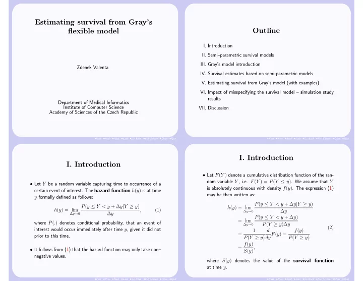
Aalen’s model with time-varying β(t)

0.0 0.1 0.2 0.3 0.4 −0.05 0.00 0.05 0.10 0.15 Time Bias 0.0 0.1 0.2 0.3 0.4 −0.05 0.00 0.05 0.10 0.15

● ● ● ●●●
0.0

0.1 0.2 0.3 0.4 −0.05 0.00 0.05 0.10 0.15 0.0 0.1 0.2 0.3 0.4 −0.05 0.00 0.05 0.10 0.15 0.0 0.1 0.2 0.3 0.4 −0.05 0.00 0.05 0.10 0.15 0.0 0.1 0.2 0.3 0.4 −0.05 0.00 0.05 0.10 0.15 0.0 0.1 0.2 0.3 0.4 −0.05 0.00 0.05 0.10 0.15

● ● ● ●●●
0.0

0.1 0.2 0.3 0.4 −0.05 0.00 0.05 0.10 0.15 Aalen

<−median survival time

0.0 0.1 0.2 0.3 0.4 −0.05 0.00 0.05 0.10 0.15 Time Bias 0.0 0.1 0.2 0.3 0.4 −0.05 0.00 0.05 0.10 0.15

● ● ● ●●●
0.0

0.1 0.2 0.3 0.4 −0.05 0.00 0.05 0.10 0.15 0.0 0.1 0.2 0.3 0.4 −0.05 0.00 0.05 0.10 0.15 0.0 0.1 0.2 0.3 0.4 −0.05 0.00 0.05 0.10 0.15 0.0 0.1 0.2 0.3 0.4 −0.05 0.00 0.05 0.10 0.15 0.0 0.1 0.2 0.3 0.4 −0.05 0.00 0.05 0.10 0.15

● ● ●
0.0

0.1 0.2 0.3 0.4 −0.05 0.00 0.05 0.10 0.15 Cox

<−median survival time

0.0 0.1 0.2 0.3 0.4 −0.05 0.00 0.05 0.10 0.15 Time Bias 0.0 0.1 0.2 0.3 0.4 −0.05 0.00 0.05 0.10 0.15

● ● ● ●●●
0.0

0.1 0.2 0.3 0.4 −0.05 0.00 0.05 0.10 0.15 0.0 0.1 0.2 0.3 0.4 −0.05 0.00 0.05 0.10 0.15 0.0 0.1 0.2 0.3 0.4 −0.05 0.00 0.05 0.10 0.15 0.0 0.1 0.2 0.3 0.4 −0.05 0.00 0.05 0.10 0.15 0.0 0.1 0.2 0.3 0.4 −0.05 0.00 0.05 0.10 0.15

● ● ● ●●●
0.0

0.1 0.2 0.3 0.4 −0.05 0.00 0.05 0.10 0.15 Gray

<−median survival time

Percentile of z

1% 10% 25% 50% 75% 90% 99% Legend 0.0 0.1 0.2 0.3 0.4 −0.5 0.0 0.5 1.0 1.5 Time MSE Relative to Aalen's model 0.0 0.1 0.2 0.3 0.4 −0.5 0.0 0.5 1.0 1.5

● ●●●
0.0

0.1 0.2 0.3 0.4 −0.5 0.0 0.5 1.0 1.5 0.0 0.1 0.2 0.3 0.4 −0.5 0.0 0.5 1.0 1.5 0.0 0.1 0.2 0.3 0.4 −0.5 0.0 0.5 1.0 1.5 0.0 0.1 0.2 0.3 0.4 −0.5 0.0 0.5 1.0 1.5 0.0 0.1 0.2 0.3 0.4 −0.5 0.0 0.5 1.0 1.5

●
0.0

0.1 0.2 0.3 0.4 −0.5 0.0 0.5 1.0 1.5 Cox

<−median survival time

0.0 0.1 0.2 0.3 0.4 −0.5 0.0 0.5 1.0 1.5 Time MSE Relative to Aalen's model 0.0 0.1 0.2 0.3 0.4 −0.5 0.0 0.5 1.0 1.5

● ● ● ●●●
0.0

0.1 0.2 0.3 0.4 −0.5 0.0 0.5 1.0 1.5 0.0 0.1 0.2 0.3 0.4 −0.5 0.0 0.5 1.0 1.5 0.0 0.1 0.2 0.3 0.4 −0.5 0.0 0.5 1.0 1.5 0.0 0.1 0.2 0.3 0.4 −0.5 0.0 0.5 1.0 1.5 0.0 0.1 0.2 0.3 0.4 −0.5 0.0 0.5 1.0 1.5

● ● ●
0.0

0.1 0.2 0.3 0.4 −0.5 0.0 0.5 1.0 1.5 Gray

<−median survival time

First •Prev •Next •Last •Go Back •Full Screen •Close •Quit

Cox PH model

0.0 0.1 0.2 0.3 0.0 0.1 0.2 0.3 0.4 Time Bias 0.0 0.1 0.2 0.3 0.0 0.1 0.2 0.3 0.4

●● ●●●
0.0

0.1 0.2 0.3 0.0 0.1 0.2 0.3 0.4 0.0 0.1 0.2 0.3 0.0 0.1 0.2 0.3 0.4 0.0 0.1 0.2 0.3 0.0 0.1 0.2 0.3 0.4 0.0 0.1 0.2 0.3 0.0 0.1 0.2 0.3 0.4 0.0 0.1 0.2 0.3 0.0 0.1 0.2 0.3 0.4

0.0

0.1 0.2 0.3 0.0 0.1 0.2 0.3 0.4 Aalen

<−median survival time censoring limit −>

0.0 0.1 0.2 0.3 0.0 0.1 0.2 0.3 0.4 Time Bias 0.0 0.1 0.2 0.3 0.0 0.1 0.2 0.3 0.4

●● ●●●
0.0

0.1 0.2 0.3 0.0 0.1 0.2 0.3 0.4 0.0 0.1 0.2 0.3 0.0 0.1 0.2 0.3 0.4 0.0 0.1 0.2 0.3 0.0 0.1 0.2 0.3 0.4 0.0 0.1 0.2 0.3 0.0 0.1 0.2 0.3 0.4 0.0 0.1 0.2 0.3 0.0 0.1 0.2 0.3 0.4

●● ●●●
0.0

0.1 0.2 0.3 0.0 0.1 0.2 0.3 0.4 Cox

<−median survival time censoring limit −>

0.0 0.1 0.2 0.3 0.0 0.1 0.2 0.3 0.4 Time Bias 0.0 0.1 0.2 0.3 0.0 0.1 0.2 0.3 0.4

●● ●●●
0.0

0.1 0.2 0.3 0.0 0.1 0.2 0.3 0.4 0.0 0.1 0.2 0.3 0.0 0.1 0.2 0.3 0.4 0.0 0.1 0.2 0.3 0.0 0.1 0.2 0.3 0.4 0.0 0.1 0.2 0.3 0.0 0.1 0.2 0.3 0.4 0.0 0.1 0.2 0.3 0.0 0.1 0.2 0.3 0.4

●● ●●●
0.0

0.1 0.2 0.3 0.0 0.1 0.2 0.3 0.4 Gray

<−median survival time censoring limit −>

0.0 0.1 0.2 0.3 10 20 30 40 50 Time MSE Relative to Cox's model 0.0 0.1 0.2 0.3 10 20 30 40 50

●● ●●●
0.0

0.1 0.2 0.3 10 20 30 40 50 0.0 0.1 0.2 0.3 10 20 30 40 50 0.0 0.1 0.2 0.3 10 20 30 40 50 0.0 0.1 0.2 0.3 10 20 30 40 50 0.0 0.1 0.2 0.3 10 20 30 40 50

0.0

0.1 0.2 0.3 10 20 30 40 50 Aalen

<− median survival time censoring limit −>

Percentile of z

1% 10% 25% 50% 75% 90% 99% Legend 0.0 0.1 0.2 0.3 10 20 30 40 50 Time MSE Relative to Cox's model 0.0 0.1 0.2 0.3 10 20 30 40 50

●● ●●●
0.0

0.1 0.2 0.3 10 20 30 40 50 0.0 0.1 0.2 0.3 10 20 30 40 50 0.0 0.1 0.2 0.3 10 20 30 40 50 0.0 0.1 0.2 0.3 10 20 30 40 50 0.0 0.1 0.2 0.3 10 20 30 40 50

●● ●●●
0.0

0.1 0.2 0.3 10 20 30 40 50 Gray

<− median survival time censoring limit −>

First •Prev •Next •Last •Go Back •Full Screen •Close •Quit

Gray’s model with time-varying β(t)

0.05 0.10 0.15 −0.1 0.1 0.2 0.3 0.4 0.5 Time Bias 0.05 0.10 0.15 −0.1 0.1 0.2 0.3 0.4 0.5

●● ● ● ● ●
● ●
0.05

0.10 0.15 −0.1 0.1 0.2 0.3 0.4 0.5 0.05 0.10 0.15 −0.1 0.1 0.2 0.3 0.4 0.5 0.05 0.10 0.15 −0.1 0.1 0.2 0.3 0.4 0.5 0.05 0.10 0.15 −0.1 0.1 0.2 0.3 0.4 0.5 0.05 0.10 0.15 −0.1 0.1 0.2 0.3 0.4 0.5

● ●
●
0.05

0.10 0.15 −0.1 0.1 0.2 0.3 0.4 0.5 Aalen

median survival time −>

0.05 0.10 0.15 −0.1 0.1 0.2 0.3 0.4 0.5 Time Bias 0.05 0.10 0.15 −0.1 0.1 0.2 0.3 0.4 0.5

●● ● ● ● ●
● ●
0.05

0.10 0.15 −0.1 0.1 0.2 0.3 0.4 0.5 0.05 0.10 0.15 −0.1 0.1 0.2 0.3 0.4 0.5 0.05 0.10 0.15 −0.1 0.1 0.2 0.3 0.4 0.5 0.05 0.10 0.15 −0.1 0.1 0.2 0.3 0.4 0.5 0.05 0.10 0.15 −0.1 0.1 0.2 0.3 0.4 0.5

●
● ●
0.05

0.10 0.15 −0.1 0.1 0.2 0.3 0.4 0.5 Cox

median survival time −>

0.05 0.10 0.15 −0.1 0.1 0.2 0.3 0.4 0.5 Time Bias 0.05 0.10 0.15 −0.1 0.1 0.2 0.3 0.4 0.5

●● ● ● ● ●
● ●
0.05

0.10 0.15 −0.1 0.1 0.2 0.3 0.4 0.5 0.05 0.10 0.15 −0.1 0.1 0.2 0.3 0.4 0.5 0.05 0.10 0.15 −0.1 0.1 0.2 0.3 0.4 0.5 0.05 0.10 0.15 −0.1 0.1 0.2 0.3 0.4 0.5 0.05 0.10 0.15 −0.1 0.1 0.2 0.3 0.4 0.5

●● ● ● ● ●
● ●
0.05

0.10 0.15 −0.1 0.1 0.2 0.3 0.4 0.5 Gray

median survival time −>

0.05 0.10 0.15 10 20 30 40 50 Time MSE Relative to Gray's model 0.05 0.10 0.15 10 20 30 40 50

●● ● ● ● ●
● ●
0.05

0.10 0.15 10 20 30 40 50 0.05 0.10 0.15 10 20 30 40 50 0.05 0.10 0.15 10 20 30 40 50 0.05 0.10 0.15 10 20 30 40 50 0.05 0.10 0.15 10 20 30 40 50

●● ● ● ● ●
0.05

0.10 0.15 10 20 30 40 50 Aalen

median survival time −>

0.05 0.10 0.15 10 20 30 40 50 Time MSE Relative to Gray's model 0.05 0.10 0.15 10 20 30 40 50

●● ● ● ● ●
● ●
0.05

0.10 0.15 10 20 30 40 50 0.05 0.10 0.15 10 20 30 40 50 0.05 0.10 0.15 10 20 30 40 50 0.05 0.10 0.15 10 20 30 40 50 0.05 0.10 0.15 10 20 30 40 50

●● ●
0.05

0.10 0.15 10 20 30 40 50 Cox

median survival time −>

Percentile of z

1% 10% 25% 50% 75% 90% 99% Legend

First •Prev •Next •Last •Go Back •Full Screen •Close •Quit
VII. Discussion
When the data satisfied Aalen’s linear model, both Cox’s a

Gray’s model rendered biased survival estimates. They have, however, often shown a lower MSE than the native model for the data at hand.

When analyzing Cox PH model data using the Gray’s rou-

tine, we observed no dramatic increase in bias and MSE relative to native model, while using the same criteria the survival esti- mates based on Aalen’s model appeared to be highly distorted.

When the data followed Gray’s model with time-varying co-

variate effects, both Cox’s and Aalen’s model rendered in terms

f bias and MSE highly unreliable estimates of the conditional

survival distribution. In other words, there was no alternative to using the native model in this instance.

SLIDE 9

First •Prev •Next •Last •Go Back •Full Screen •Close •Quit

References

[1] Cox DR: Regression Models and Life Tables (with discussion), Journal of the Royal Statistical Society, 1972, Vol. 34, pp. 187–220. [2] Aalen OO: A linear regression model for the analysis of life times, Statistics in Medicine, 1989, Vol. 8, pp. 907–925. [3] Gray RJ: Flexible methods for analyzing survival data using splines, with ap- plication to breast cancer prognosis, Journal of the American Statistical Associ- ation, 1992, Vol. 87, pp. 942–951. [4] Gray RJ: Spline-based tests in survival analysis, Biometrics, 1994, Vol. 50., pp. 640–652. [5] Valenta Z and Weissfeld LA: Estimation of the Survival Function for Gray’s Piecewise-Constant Time-Varying Coefficients Model, Statistics in Medicine, 2002, Vol. 21(5), pp. 717-727.

First •Prev •Next •Last •Go Back •Full Screen •Close •Quit