Previous Lecture Slides for Lecture 6 ENCM 501: Principles of - - PDF document

Slides for Lecture 6

ENCM 501: Principles of Computer Architecture Winter 2014 Term Steve Norman, PhD, PEng

Electrical & Computer Engineering Schulich School of Engineering University of Calgary

28 January, 2014

ENCM 501 W14 Slides for Lecture 6

slide 2/33

Previous Lecture

◮ introduction to ISA design ideas ◮ memory-register and load-store architectures ◮ a very brief history of RISC versus CISC ◮ aspects of the ISA view of memory—flat address spaces,

alignment rules

ENCM 501 W14 Slides for Lecture 6

slide 3/33

Today’s Lecture

◮ endianness ◮ addressing modes ◮ examples of tradeoffs in instruction set design

Related reading in Hennessy & Patterson: Sections A.3–A.7

ENCM 501 W14 Slides for Lecture 6

slide 4/33

Endianness

This is not really an aspect of computer design in which there are interesting cost or performance tradeoffs. Rather, it’s an annoying detail that will occasionally bite you if you aren’t aware of it. Registers inside processor cores do not have endianness. An N-bit register just has bits N−1 (MSB), N−2, . . . , 2, 1, 0 (LSB). Endianness is a property of the interface between the processor core and the memory, and comes from the fact that most ISAs allow memory reads and writes with various sizes, typically 1-byte, 2-byte, 4-byte, and 8-byte.

ENCM 501 W14 Slides for Lecture 6

slide 5/33

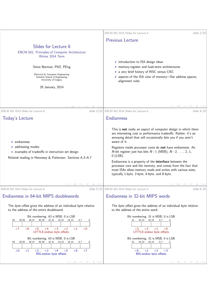
Endianness in 64-bit MIPS doublewords

The byte offset gives the address of an individual byte relative to the address of the entire doubleword.

+7 +6 +5 +4 +3 +2 +1 +0

63 56 55

Bit numbering: 63 is MSB, 0 is LSB

48 47 40 39 32 31 24 23 16 15 8 7

LITTLE-endian byte offsets

63 56 55

Bit numbering: 63 is MSB, 0 is LSB

48 47 40 39 32 31 24 23 16 15 8 7

BIG-endian byte offsets +0 +1 +2 +3 +4 +5 +6 +7

ENCM 501 W14 Slides for Lecture 6

slide 6/33

Endianness in 32-bit MIPS words

The byte offset gives the address of an individual byte relative to the address of the entire word.

24 23 16 15 8 7 24 23 16 15 8 7

+3 +2 +1 +0 Bit numbering: 31 is MSB, 0 is LSB

31

LITTLE-endian byte offsets +0 +1 +2 +3 BIG-endian byte offsets Bit numbering: 31 is MSB, 0 is LSB

31

ENCM 501 W14 Slides for Lecture 6

slide 7/33

Example effect of endianness in MIPS32

# LI: pseudoinstruction # for "load immediate" LI R9, 0x12345678 SW R9, 0(R8) LB R10, 0(R8) LB R11, 1(R8) LB R12, 2(R8) LB R13, 3(R8) Assume that R8 contains some valid address that is a multiple of four. What goes into R10, R11, R12, R13, if the processor chip is in little-endian mode? What if the processor chip is in big-endian mode?

ENCM 501 W14 Slides for Lecture 6

slide 8/33

Practical code rarely (if ever) writes data as a word and later reads it back as bytes, as was done in the example on the last

• slide. Why is endianness a practical concern?

Here is a practical problem:

◮ Program P1 on Computer C1 copies an array of integers

• r FP numbers from memory into a file using a function

like fwrite in the C library.

◮ On disk, the file is just a long sequence of bytes. ◮ Program P2 on Computer C2 opens the file and tries to

read the array of numbers from the file into memory using a function like fread in the C library.

◮ But C2 does not have the same endianness as C1, so the

data does not make sense to P2. The same kind of problem can happen when streaming multi-byte numbers over a network.

ENCM 501 W14 Slides for Lecture 6

slide 9/33

Endianness and real systems

Today little-endianness is much more common than big-endianness. Here are some little-endian systems:

◮ anything running on x86 or x86-64; ◮ Apple iOS, Linux (including Android), and Windows

running on ARM. Some historically important big-endian machines were:

◮ Macs with 68000- or PowerPC-based processors; ◮ 68000- and SPARC-based computers from Sun

Microsystems. Many modern ISA families, for example, MIPS and ARM, allow the processor to switch back and forth between little- and big-endian modes.

ENCM 501 W14 Slides for Lecture 6

slide 10/33

Addressing modes

Unlike endianness, selection of addressing modes for an ISA is a set of design decisions that involve interesting tradeoffs. Addressing mode is a slightly misleading term, because it refers to the way in which an operand is accessed by an instruction, and that might or might not involve generation

• f a memory address.

Addressing modes for data access are discussed as part of Section A.3 in the textbook. Addressing modes for instruction access—needed, for example, by branches and jumps—are discussed in Section A.6.

ENCM 501 W14 Slides for Lecture 6

slide 11/33

Examples of addressing modes for data

Figure A.6 in the textbook gives examples covering most addressing modes available in ISAs of the present and the recent past. A typical ISA will support some but not all of these addressing modes. (Historical note: I think the MC68000 series supported all of them and more, which is kind of awesome.) This lecture won’t explain every addressing mode in detail, but instead will look at the ones that are most common and

• important. Let’s start with the two modes that don’t involve

generation of a memory address . . .

ENCM 501 W14 Slides for Lecture 6

slide 12/33

Addressing modes: Register and Immediate

Register: Data is coming from or going to a register. All three operands are accessed in register mode in this MIPS64 instruction: DADDU R10, R8, R9 Immediate: Source data is a constant written into the

• instruction. Here is a MIPS64 example in which two operands

are register-mode and one is immediate-mode: DADDIU R16, R16, 8

ENCM 501 W14 Slides for Lecture 6

slide 13/33

Encoding of immediate operands in example ISAs

x86-64: Instruction size is variable, so 1, 2, 4, or 8 bytes are used, as necessary, to describe the constant. MIPS32 and MIPS64: Instructions are always 32 bits wide and the field size for immediate operands is always 16 bits

• wide. The range of constants is −32768 to +32767 for

instructions that use signed constants and 0 to 65535 for those that use unsigned constants. ARM: 12 bits within the fixed instruction size of 32 bits are used for an immediate operand, in a complicated and interesting way that could totally derail a lecture! (That’s one

• f a few very good reasons why it would not be easy to switch

from MIPS to ARM in ENCM 369.)

ENCM 501 W14 Slides for Lecture 6

slide 14/33

The two simplest addressing modes for memory access

Hint for comprehension: Roughly speaking, indirect means “via a pointer”. Register indirect: Use the bits in a register as a memory

• address. MIPS64 example:

LD R8, (R9) # R8 = doubleword at address in R9 Displacement: Add a constant to the bits in a register to generate a memory address. MIPS64 example: # R10 = doubleword at address R10 + 64 bytes LD R10, 64(R11) Why is register indirect mode really just a special case of displacement mode?

ENCM 501 W14 Slides for Lecture 6

slide 15/33

Scaled mode: Good for array element access

Here is some x86-64 assembly language code you will look at in Assignment 2 . . . .L16: mov (%rbx,%rax,4), %edx addq $1, %rax addq %rdx, %rbp cmpq $500000000, %rax jne .L16 The mov instruction uses scaled mode: The address used to read memory is %rbx + 4 × %rax %rbx is the address of element 0 of an array of 4-byte elements, and %rax is an index into that array.

ENCM 501 W14 Slides for Lecture 6

slide 16/33

Autoincrement and autodecrement modes (1)

Other names for these modes are post-increment and pre-decrement. In either of these modes a load causes two register updates—one to a destination register, and another to a pointer register. A store also causes two updates—one update to a memory location and another to a pointer register. Both are useful for walking through arrays using pointer arithmetic. A store using pre-decrement mode is an efficient way to push a register value on to a stack. And a load using post-increment mode is an efficient way to pop a register value from a stack.

ENCM 501 W14 Slides for Lecture 6

slide 17/33

Autoincrement and autodecrement modes (2)

These modes closely match some famously tricky C and C++ expressions. Let’s write a couple of C statements that could be each be implemented using a single instruction if autoincrement and autodecrement modes are available.

ENCM 501 W14 Slides for Lecture 6

slide 18/33

Memory indirect mode

Example, using syntax from textbook Figure A.6: MOV R0, @(R1) The address in R1 is used to read a second address from memory. That second address is used to read from memory into R0. In a typical load/store architecture this would be done with two instructions: a load followed by another load. Another example, using the same syntax: MOV @(R2), R3 The address in R2 is used to read a second address from memory. That second address is used to write the data from R3 to memory. In a typical load/store architecture this would be done with two instructions: a load followed by a store. This mode is somewhat obsolete these days, but thinking about it helps to understand pointer-to-pointer types in C and C++.

ENCM 501 W14 Slides for Lecture 6

slide 19/33

MIPS instruction format for loads and stores

Just about all MIPS32 and MIPS64 load and store instructions are organized like this:

• pcode

31 26 25 21 20 16 15

base rt

• ffset

There are various different opcodes for loads and stores of various sizes of data. The address is formed by adding the sign-extension of the 16-bit offset and the address in GPR

• base. rt is the source register for a store and and the

destination register for a load. The addressing mode for memory is displacement. What are some advantages and disadvantages of offering only displacement mode for loads and stores?

ENCM 501 W14 Slides for Lecture 6

slide 20/33

What limits the number of GPRs (or FPRs) available to an ISA?

The limit is not due to the chip area dedicated to registers! For example, MIPS64 has 32 64-bit GPRs, which is a larger than typical number of GPRs for current ISAs. MIPS64 requires an array of 32 × 64 one-bit cells, that is, 211 = 2048 bits, or 256 bytes. Currently, L1 caches are 32 kB or larger—much, much bigger than 256 bytes. So why are ISAs with large number of GPRs—say, 64, or 256,

• r 1024—quite uncommon?

ENCM 501 W14 Slides for Lecture 6

slide 21/33

Load and store word examples in ARM7TDMI

Here is one of many formats for instructions to load or store 32-bit words:

31 16 15

cond

28 27 4 3

Rm

12 11 20 19 24 23

0111 001 Rn Rd

5

The above pattern is for load. Change bit 20 to 0 for store. Rd gives the destination GPR for load, and source GPR for

• store. The memory address is computed using two GPRs, Rn

and Rm, plus, in a complicated way, constants encoded in bits 23 and 11–5. Essentially, this particular format allows numerous variations of scaled addressing mode.

ENCM 501 W14 Slides for Lecture 6

slide 22/33

Warning: The details are quite complex, so I possibly have some of them wrong! Mistakes or not, the contrast with MIPS is striking. Various other ARM load and store formats allow every addressing mode in textbook Figure A.6—except memory indirect—and some interesting combinations of those modes. What advantages are there to the huge variety of ARM load and store formats, compared to the distinct lack of variety in MIPS load and store formats? What disadvantages might there be? Note: Every ARM instruction starts with a 4-bit cond field. We’ll get to that soon.

ENCM 501 W14 Slides for Lecture 6

slide 23/33

Instructions for control flow

As discussed in textbook Section A.6, this category includes

◮ conditional branches ◮ jumps ◮ procedure calls ◮ procedure returns

In general, these are instructions that might (conditional branch) or will (the others) cause a special update to the PC (program counter register).

ENCM 501 W14 Slides for Lecture 6

slide 24/33

Target instructions and target addresses

A useful term related to control flow is target instruction, which is

◮ in the case of conditional branch, the first instruction

executed after a branch is taken—a branch is taken or not taken depending on whether some condition is true;

◮ in the cases of jumps, calls, and returns, the first

instruction executed as a result of a jump, call, or return instruction. The target address is simply the address of the target instruction.

ENCM 501 W14 Slides for Lecture 6

slide 25/33

Addressing modes for control flow instructions

Addressing modes for control flow instructions are essentially just methods for generating target addresses. For branches, jumps, and calls, the most common addressing mode is PC-relative, in which an offset is extracted from the instruction and added to the current PC value. In MIPS and ARM the offsets in PC-relative instructions are numbers of instructions, but in x86 and x86-64 the offset is a number of bytes. Why is there a difference here? Why would PC-relative addressing not work in procedure return instructions?

ENCM 501 W14 Slides for Lecture 6

slide 26/33

Conditional branch options

Most ISAs make branch decisions based on a few bits called flag bits or condition code bits that sit within some kind of processor status register. Let’s look at this for a simple C example, in which j and k are int variables in registers: if (i < k) goto L1; x86-64 translation, assuming i in %eax, k in %edx: cmpl %edx, %eax # compare registers jl L1 # branch based on N and V flags jl means “jump if less than.” (Note: In reality the assembly language label almost certainly won’t be the same as the C label L1.)

ENCM 501 W14 Slides for Lecture 6

slide 27/33

For the same C code, here is an ARM translation, assuming i in r0, k in r1: CMP r0, r1 ; compare registers BLT L1 ; branch based on N and V flags MIPS is unusual—the comparison result goes into a GPR. Suppose we have i in R4, k in R5 . . . SLT R8, R4, R5 # R8 = (R4 < R5) BNE R8, R0, L1 # branch if R8 != 0

ENCM 501 W14 Slides for Lecture 6

slide 28/33

Conditional instructions in ARM

Recall from Assignment 1 that MIPS offers the conditional move instructions MOVN and MOVZ. (MIPS also has some similar floating-point conditional move instructions). ARM takes this idea to the extreme—every ARM instruction is conditional! Bits 31–28 of an ARM instruction are the so-called cond field, which specifies that the instruction either performs some action or is a no-op, depending on some condition on zero or more of the N, Z, V and C flags. Example ARM cond field patterns:

◮ 1110, for ALWAYS. The instruction is never a no-op.

This is the default cond field in ARM assembly language.

◮ 0000, for EQUAL. Execute the instruction if and only if

the Z flag is 1.

ENCM 501 W14 Slides for Lecture 6

slide 29/33

The power of ARM conditional instructions is illustrated by this example . . . Here is some C code: if (i == 33 || i == 63) count++; If i and count are ints in ARM registers r0 and r1, here is ARM assembly language for the C code: TEQ r0, #33 ; # indicates immediate mode TEQNE r0, #63 ADDEQ r1, #1, #1 The cond field for the first instruction is 1110, for “always”. For the second instruction, it’s 0001, for “do it only if the Z flag is 0”, and for the third, it’s 0000, for “do it only if the Z flag is 1”.

ENCM 501 W14 Slides for Lecture 6

slide 30/33

Acknowledgment: Example on previous slide adapted from an example on pages 129–130 of Hohl, W., ARM Assembly Language: Fundamentals and Techniques, c 2009, ARM (UK), published by CRC Press.

ENCM 501 W14 Slides for Lecture 6

slide 31/33

MIPS versus ARM: Vague arguments

CPU time = IC × CPI × clock period MIPS attacks CPI by making instructions very simple and easy to pipeline. ARM tries to be close to MIPS with respect to CPI, and is much better than older CISC ISAs for CPI. ARM attacks IC by doing things in one instruction that might sometimes take two

• r three MIPS instructions.

ENCM 501 W14 Slides for Lecture 6

slide 32/33

MIPS versus ARM: How to be quantitative

A fair and thorough study would require at least:

◮ real applications that are reasonably good fits for both

ISAs;

◮ the best possible compilers for each of the ISAs; ◮ processors fabricated with the same transistor and

interconnect technology, and very similar die sizes. Even then, it might not be a truly fair fight between ISAs, if

• ne side has better digital designers than the other.

ENCM 501 W14 Slides for Lecture 6

slide 33/33

Upcoming Topics

◮ The memory hierarchy

Related reading in Hennessy & Patterson: Appendix B