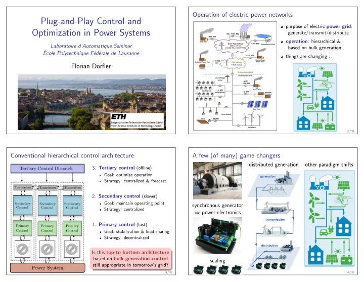
Plug-and-Play Control and purpose of electric power grid : - PowerPoint PPT Presentation

Operation of electric power networks Plug-and-Play Control and purpose of electric power grid : Optimization in Power Systems generate/transmit/distribute operation : hierarchical & Laboratoire d’Automatique Seminar based on bulk generation ´ Ecole Polytechnique F´ ed´ erale de Lausanne things are changing . . . Florian D¨ orfler 2 / 32 Conventional hierarchical control architecture A few (of many) game changers distributed generation other paradigm shifts 3. Tertiary control (offline) Goal: optimize operation generation ! Strategy: centralized & forecast 2. Secondary control (slower) Goal: maintain operating point synchronous generator Strategy: centralized ⇒ power electronics transmission ! 1. Primary control (fast) Goal: stabilization & load sharing Strategy: decentralized distribution ! Is this top-to-bottom architecture based on bulk generation control scaling still appropriate in tomorrow’s grid? Power System 3 / 32 4 / 32

Challenges & opportunities in tomorrow’s power grid A preview – plug-and-play operation architecture flat hierarchy, distributed, no time-scale separations, & model-free . . . � perational challenges ◮ more uncertainty & less inertia source # 2 source # 1 source # n ◮ more volatile & faster fluctuations … … Tr ansceiver Transceiver Transceiver … � pportunities Second ary Second ary Second ary Ter tiary T e rtiary T e rtiary Control Control Control ◮ re-instrumentation: comm & sensors Control Control Control and actuators throughout grid ◮ advances in control of cyber- Pr imary Pr imary Pr imary physical & complex systems Control Control Control ◮ break vertical & horizontal hierarchy Power System ◮ plug’n’play control: fast, model-free, & without central authority Power System 5 / 32 6 / 32 Outline Introduction Modeling Primary Control Tertiary Control Secondary Control modeling & assumptions P-n-P Experiments Beyond Emulation & PID Conclusions we will illustrate all theorems with experiments

Modeling: a power system is a circuit Modeling: a power system is a circuit 1 synchronous AC circuit with 1 synchronous AC circuit with harmonic waveforms E i e i( θ i + ω ∗ t ) harmonic waveforms E i e i( θ i + ω ∗ t ) j j i i G ij + i B ij G ij + i B ij i i 2 loads demand constant power 2 loads demand constant power P ∗ i + i Q ∗ P ∗ i + i Q ∗ i i injection = � injection = � 3 coupling via Kirchhoff & Ohm 3 coupling via Kirchhoff & Ohm power flows power flows 4 identical lines G / B = const . 4 identical lines G / B = const . (equivalent to lossless case G / B = 0) (equivalent to lossless case G / B = 0) 5 decoupling: P i ≈ P i ( θ ) & Q i ≈ Q i ( E ) 5 decoupling: P i ≈ P i ( θ ) & Q i ≈ Q i ( E ) (for simplicity of presentation) (for simplicity of presentation) � � ◮ active power: ◮ trigonometric active power flow: P i = j B ij E i E j sin( θ i − θ j ) + G ij E i E j cos( θ i − θ j ) P i ( θ ) = j B ij sin( θ i − θ j ) Q i = − � = − � ◮ reactive power: ◮ polynomial reactive power flow: j B ij E i E j cos( θ i − θ j ) + G ij E i E j sin( θ i − θ j ) Q i ( E ) j B ij E i E j (not today) 7 / 32 7 / 32 Modeling the “essential” network dynamics & controls (models can be arbitrarily detailed) 1 synchronous machines (swing dynamics) me ch. electr. M i ¨ i + P c θ i = P ∗ i − P i ( θ ) torqu e torque primary control 2 DC & variable AC sources interfaced with voltage-source converters (droop characteristic) Ee i( θ + ω t ) P ∗ i + P c i = P i ( θ ) P i ( θ ) , Q i ( E ) 3 controllable loads (voltage- and frequency-responsive) P i + i Q i P ∗ i + P c i = P i ( θ ) Ee i( θ + ω t ) 8 / 32

Decentralized primary control of active power Putting the pieces together... differential-algebraic, nonlinear, large-scale closed loop Emulate physics of dissipative 50 49 51 n e twork physics 48 52 coupled synchronous machines : power c onsumed power supplied P mech i + P c power balanc e: = P ∗ i − P i ( θ ) M i ¨ θ + D i ˙ i θ i � j B ij si n( θ i − θ j ) power flow: P i ( θ ) = Hz � = P ∗ i − j B ij sin( θ i − θ j ) droop control D i ˙ θ i = ( P ∗ i − P i ( θ )) Conventional wisdom: physics ω sync = � i / � i P ∗ are naturally stable & sync fre- i D i quency reveals power imbalance � M i ¨ θ i + D i ˙ θ i = P ∗ synchronous machines: i − j B ij sin( θ i − θ j ) � D i ˙ P / ˙ θ i = P ∗ inverter sources: i − j B ij sin( θ i − θ j ) θ droop control: ( ω i − ω ∗ ) ∝ ( P ∗ i − P i ( θ )) � D i ˙ θ i = P ∗ i − j B ij sin( θ i − θ j ) controllable loads: � ω sync � D i ˙ θ i = P ∗ 0 = P ∗ i − P i ( θ ) passive loads/inverters: i − j B ij sin( θ i − θ j ) 9 / 32 10 / 32 Closed-loop stability under droop control Theorem: stability of droop control [J. Simpson-Porco, FD, & F. Bullo, ’12] ∃ unique & exp. stable frequency sync ⇐ ⇒ active power flow is feasible Main proof ideas and some further results : tertiary control � i + � sources P ∗ loads P ∗ ω sync = ω ∗ + i • synchronization frequency: � sources D i ( ∝ power balance) (energy management) � P ∗ (# i passive) i • steady-state power injections: P i = P ∗ i − D i ( ω sync − ω ∗ ) (# i active) (depend on D i & P ∗ i ) • stability via incremental Lyapunov [Zhao, Mallada, & FD ’14, J. Schiffer & FD ’15] V ( x ) = kinetic energy + DAE potential energy + ε · Chetaev cross term 11 / 32

Tertiary control & energy management Tertiary control & energy management an offline resource allocation & scheduling problem an offline resource allocation & scheduling problem minimize { cost of generation, losses, . . . } subject to equality constraints: power balance equations inequality constraints: flow/injection/voltage constraints logic constraints: commit generators yes/no . . . 12 / 32 12 / 32 Objective: economic generation dispatch Objective: decentralized dispatch optimization minimize the total accumulated generation (many variations possible) Insight: droop-controlled system = decentralized primal/dual algorithm � sources α i u 2 minimize θ ∈ T n , u ∈ R nI J ( u ) = i Theorem: optimal droop [FD, Simpson-Porco, & Bullo ’13, Zhao, Mallada, & FD ’14] subject to The following statements are equivalent: P ∗ source power balance: i + u i = P i ( θ ) P ∗ load power balance: i = P i ( θ ) (i) the economic dispatch with cost coefficients α i is strictly feasible with global minimizer ( θ ⋆ , u ⋆ ). branch flow constraints: | θ i − θ j | ≤ γ ij < π/ 2 (ii) ∃ droop coefficients D i such that the power system possesses a α i u ⋆ i = α j u ⋆ Unconstrained case: identical marginal costs at optimality unique & locally exp. stable sync’d solution θ . j If (i) & (ii) are true, then θ i ∼ θ ⋆ i , u ⋆ i = − D i ( ω sync − ω ∗ ), & D i α i = D j α j . In conventional power system operation, the economic dispatch is solved offline , in a centralized way, & with a model & load forecast similar results for non-quadratic (strictly convex) cost & constraints In a grid with distributed energy resources, the economic dispatch should be similar results in transmission ntwks with DC flow [E. Mallada & S. Low, ’13] solved online , in a decentralized way, & without knowing a model & [N. Li, L. Chen, C. Zhao, & S. Low ’13] & [X. Zhang & A. Papachristodoulou, ’13] & [M. Andreasson, D. V. Dimarogonas, K. H. Johansson, & H. Sandberg, ’13] & . . . 13 / 32 14 / 32