
SLIDE 1
Perception of Motion
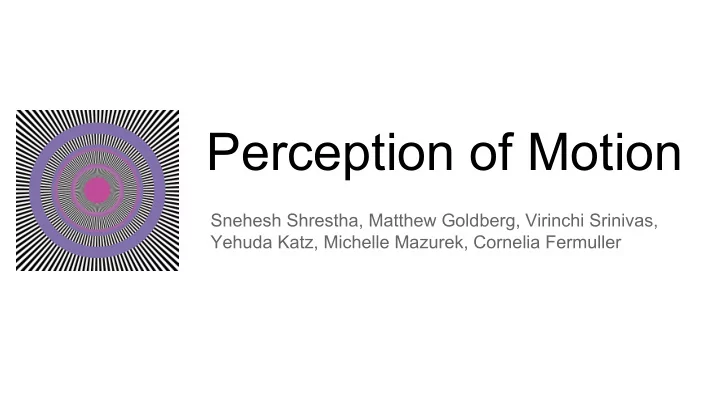
Snehesh Shrestha, Matthew Goldberg, Virinchi Srinivas, Yehuda Katz, Michelle Mazurek, Cornelia Fermuller
Perception of Motion Snehesh Shrestha, Matthew Goldberg, Virinchi - - PowerPoint PPT Presentation
Perception of Motion Snehesh Shrestha, Matthew Goldberg, Virinchi Srinivas, Yehuda Katz, Michelle Mazurek, Cornelia Fermuller Introduction Optical Illusions such as Leviant Illusion Observation Spinning/ Flickering motion in
Perception of Motion
Snehesh Shrestha, Matthew Goldberg, Virinchi Srinivas, Yehuda Katz, Michelle Mazurek, Cornelia Fermuller
Introduction
Illusion
○ Spinning/ Flickering motion in static images ○ Believed universal
○ Angle of intersection (~90o) ○ Density of lines
Motivation
Problems
done
Experiment Goals:
○ Time taken ○ Angles of intersection ○ Density of ■ Number of lines ■ Ratio of lines and space between them
METHODS: Experiment Design
at random.
(something moving) in the image
○ Baseline reaction time ○ Random images of cars, scenery, and random patterns known to not have illusions are shown
do they see, screen resolution, demographics are collected
METHODS: Design / Interface / Pilot
1. Experiment design
a. Web survey - Reach large audience fast b. Keyboard Control - less variability
2. Web interface and backend - Python/Flask, MySQL, Piwik Analytics 3. Illusion images - Generated in Matlab 4. Pilot - Friends and family
a. Observed and collected feedback b. Updated the interface, images etc based on the pilot.
Experiment Setup: Reaction Time Baseline
Experiment Setup: Data
METHODS: Recruitment
1. Social media
a. Facebook b. LinkedIn c. Twitter
2. Email
a. Community and University Email Lists b. Emails to friends and family
3.
Flyers
4.
MTurk a. Threat to validity b. Worldwide representative sample
5.
METHODS: Analysis
○ Does variation in angles/line density/ line space ratio affect the reaction time to observe any illusion?
○ Variation in angles / line density / line space ratio is not related to reaction time to observe any illusion
○ No difference in reaction time on varying angles / line density / line space ratio
METHODS: Analysis
○ Does Age, Race, Gender and optical defect affect the possibility of observing illusion?
○ Age, Race, Gender and optical defect are not related to the possibility of observing illusion.
in general troublesome to assess for categorical cases for all IV
METHODS: Limitations
○ Requires between 97 and 117 samples for hypotheses testing relation between density, angles, spacing vs time ○ Requires 140 samples for hypothesis involving multiple linear regression
METHODS: Assumption
race, optical deficiencies etc. do not have effect on each other
RESULTS:: Variation: Density of Lines-Space Ratio
4 2 8 16 RESULTS: Hypothesis (1a): Ratio of lines-space
hypothesis test: p-value = 2.08e-12
The distribution is uniform
histograms as well
RESULTS:: Variation: Density of Lines
RESULTS:: Variation: Density of Lines
=2 2 4 8 32 96 120 RESULTS: Hypothesis (1b): Number of lines
hypothesis test: p-value < 2.2e-16
Distribution is uniform
identically distributed
RESULTS:: Variation: Angles
RESULTS: Hypothesis (1c) : Angles
hypothesis test: p-value = 0.9637
hypothesis unaffected
examination of distribution location
RESULTS: Hypothesis (2): Demographics
lm(formula = one ~ AgeGroup + Gender + Race + lensGroup, data = new_data) Residuals: Min 1Q Median 3Q Max RESULTS: Demographics Distribution: VISITORS
Total Participants 260 Valid Participants 67
RESULTS: Demographics Distribution: RACE
RESULTS: Demographics Distribution: GENDER
RESULTS: Corrective Lens Effect
RESULTS: Demographics Distribution: AGE
RESULTS: Age vs Reaction & Illusion Seeing Time
DISCUSSION and CONCLUSION
1. Results show that changes in density is related to how fast and more people observing the illusion. Changes in angles does not seem to affect. 2. There were many challenges, however, we learned a lot and esp. How to reduce the risk to validity to our tests. 3. Even though we did not have sufficient samples, the results look promising and with lessons learned from this full process, we can use this as a pilot and conduct a larger and stronger experiment. 4. Future work: This summer we plan to continue this work under Dr. Fermuller and Dr. Mazurek's guidance.
Q&A
Thank You!
Histogram of did NOT see across different params
RESULTS: Did NOT see distribution
Rough outline for to follow
1. Intro/Motivation/ Background 2. Method Details
a. Overview/ Plan b. Design/ Interface/ Pilot c. Recruitment d. Methods analysis (Assumptions…)
3. Results
a. Data Overview (distribution, results of the tests and interpretations) b. Discussion on the hypothesis
4. Discussions
a. Implication of the results b. Limitations (Challenges, …) c. Next Steps/ Future Work d. Lessons Learned from this study as pilot (Coulda/Shouda, ...)
5. Conclusion