overview lists recursive functions in lambda calculus equational - PowerPoint PPT Presentation

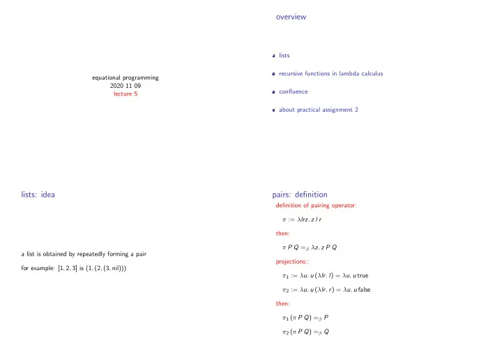
overview lists recursive functions in lambda calculus equational programming 2020 11 09 confluence lecture 5 about practical assignment 2 lists: idea pairs: definition definition of pairing operator: π := λ lrz . z l r then: π P Q = β λ z . z P Q a list is obtained by repeatedly forming a pair projections:: for example: [1 , 2 , 3] is (1 , (2 , (3 , nil))) π 1 := λ u . u ( λ lr . l ) = λ u . u true π 2 := λ u . u ( λ lr . r ) = λ u . u false then: π 1 ( π P Q ) = β P π 2 ( π P Q ) = β Q

lists: definition empty constructors: nil := λ xy . y how do we define a predicate isempty on lists? cons := λ ht . λ z . z h t = π definition: cons H T = β λ z . z H T head := λ l . l ( λ ht . h ) = π 1 nil := λ xy . y tail := λ l . l ( λ ht . t ) = π 2 isempty := λ l . l ( λ x .λ y .λ z . false) true then: head (cons H T ) = β H tail (cons H T ) = β T additional work on encodings overview lists paper about numerical systems in lambda-calculus by Ian Mackie recursive functions in lambda calculus paper about data types in lambda-calculus by Herman Geuvers confluence and the references in those papers about practical assignment 2

recursive functions: examples in Haskell how do we define length in lambda-calculus? first idea: factorial n = if (n==0) then 1 length = λ l . if l is empty then zero, else length of tail of l plus 1 else (n * factorial (n-1)) lists represented as nil := λ xy . y and cons := λ ht . λ z . z h t conditional represented as ite = λ b . λ x .λ y . b x y som [] = 0 check on empty represented as isempty := λ l . l ( λ xyz . false) true som (h:t) = h + (som t) Church numerals with 0 represented as c 0 = λ s . λ z . z tail represented as tail = λ l . l ( λ h . λ t . t ) length [] = 0 length (h:t) = (length t) + 1 plus one represented as S = λ x . λ sz . s ( x s z ) use fixed point combinator to define recursive functions recursive functions: method we try to define: So far we have: G with G = . . . G . . . length := λ l . ite (isempty l ) c 0 (S (length (tail l ))) which still contains length. Now using hence we look for: G with G = ( λ g . . . . g . . . ) G M := λ a . λ l . ite (isempty l ) c 0 (S ( a (tail l ))) we have hence we take: length = β M length a fixed point of λ g . . . . g . . . So we actually look for a fixed point of M ! So we take: length := Y M that is, using a fixed point combinator Y we define: with M defined as above, and Y Curry’s fixed point combinator G = Y ( λ g . . . . g . . . )

from Haskell to lambda remark: lambda calculi with patterns Haskell is translated to core Haskell which can be seen as λ + length [] = 0 computation by reduction and pattern matching: length (h:t) = (length t) + 1 becomes first projection: ( λ � x , y � . x ) � 3 , 5 � → x [ x , y := 3 , 5] = 3 length l = case l of [] -> 0 length of a non-empty list: (h:t) -> 1 + length t ( λ ( h : t ) . 1 + (length t )) (1 : nil) → (1 + (length t ))[ t := nil] = 1 + length nil becomes (...) becomes roughly Y ( λ a . λ l . if ( l == []) then 0 else ( λ ( h : t ) . (1 + ( a t ))) l ) overview a next question lists we know what is a result (normal form or weak head normal form) recursive functions in lambda calculus we know how to get there (leftmost-outermost reduction) this is a way of dealing with non-termination confluence but we may also use a different evaluation, do we then get the same result? about practical assignment 2 that is: what can we say about non-determinism?

side effects and unique results lazy evaluation and unique results if side-effects are present we may obtain different results n + (n:=1) = { use (initial) value 0 for n } 0 + (n:= 1) = { perform assignment for n} every two terminating evaluations of the same Haskell expression 0 + 1 = { apply + } yield the same result 1 whereas the following evaluation yields another result: we will discuss this issue in the pure λ -calculus n + (n:=1) = { perform assignment for n } n + 1 = { use (new) value 1 for n } 1 + 1 = { apply + } 2 Koblenz confluence: what and why what is confluence? intuition: two coinitial diverging computations can be joined why is it useful? because it gives unicity of normal forms is λ -calculus with β -reduction confluent? yes how do we prove confluence?

confluence of beta-reduction: definition example of a non-confluent system intuition: two coinitial diverging computations can be joined definition: a c b d if M → ∗ β N and M → ∗ β N ′ β P and N ′ → ∗ then there exists P with N → ∗ β P the definition can be given in general for a reduction relation → why is confluence useful? confluence for lambda-calculus with beta-reduction Assume → is confluent. theorem: λ -calculus with β -reduction is confluent Let N be a normal form of P , consequence: that is: P reduces to N and N cannot do a step. a λ -term has at most one β -normal form (why?) Suppose also M is a normal form of P , consequence: that is: P reduces to M and M cannot do a step. if M = β N then there exists P with M → ∗ β P and N → ∗ β P (why?) then N and M are equal (modulo α ) (why?) consequence of consequence: lambda equality is not trivial, example: λ x . λ y . x � = β λ x . λ y . y confluence implies that the normal form of a term is unique

informal equational reasoning: example divergence informal equational reasoning: example divergence we use the definition double x = x + x . we use the definition double x = x + x double (double 2) double (double 2) = { unfold definition OUTER double } = { unfold definition INNER double } (double 2) + (double 2) double (2 + 2) = {unfold definition left double } = {unfold definition double } (2 + 2) + (double 2) (2 + 2) + (2 + 2) = {apply first +} = {apply first +} 4 + (double 2) 4 + (2+2) = {unfold definition double} = {apply last +} 4 + (2+2) 4 + 4 = {apply second +} = {apply +} 4+ 4 8 = {apply +} 8 lambda-calculus: example divergence pure and impure functional programming languages pure: Haskell, Miranda programs are pure mathematical functions pure equational reasoning • ( λ x . ( λ y . f y y ) x ) ( I z ) → β ( λ x . f x x ) ( I z ) → β f ( I z ) ( I z ) no side effects • ( λ x . ( λ y . f y y ) x ) ( I z ) → β ( λ x . ( λ y . f y y ) x ) z impure: ML, Scheme possible side effects, for example assigment and exceptions more difficult to reason about

overview programming assignment 2 lists infinite lists using lazy evaluation recursive functions in lambda calculus Church numerals confluence algebraic data types monads about practical assignment 2 monads lambda and Haskell: data types we can write for example Church numerals in Haskell (prac 2)) churchnumeral n = if (n==0) then \s -> \z -> z else \s -> \z -> (churchnumeral (n-1) s (s z)) simulate in a pure setting side effects now called actions also: algebraic data types in Haskell encounter with monads in the practical work example: booleans data Bool = False | True deriving (Eq, Show) no monads in the written exam more general paper by Philip Wadler about monads example: natural numbers data Nat = Zero | Suc Nat deriving (Eq, Show) example: polymorphically labelled binary tree: data Binarytree a = Leaf | Node (Binarytree a) a (Binarytree a) deriving Show