X E Y (1) Z (2) Z (3) Z Exact inference by enumeration - - PowerPoint PPT Presentation

SLIDE 1 ✁ ✂ ✄ ☎✆ ✝✞ ✂ ✟ ☎ ✁ ✂ ☎ ✠ ✄ ✂ ✟✡ ✞ ✟ ☛ ☞ ✁ ✂✌ ☞ ☞ ✟ ✍ ✌ ✁ ✞ ✌ ✎✏✑ ✒ ✓ ✒ ✏ ✔ ✒ ✕ ✏ ✖ ✒ ✗ ✕ ✒ ✑ ✏ ✒✘✙ ✚ ✓✛ ✜ ✢ ✣ ✤ ✥ ✦✧ ★✩ ✪ ✫✬ ✭ ✮ ✯ ✰ ✧ ✱ ✲ ✳✴✵ ✴✶ ✷ ✸✹ ✺ ✻✼✽✾ ✿ ❀❁ ❂❃ ❁ ❄ ❅❆ ✾ ✽ ✼ ❇ ❈ ❄ ❉ ❊ ❋ ✼ ✼ ✽ ❅ ❅ ✻ ❀ ✾

• ❉❍

✿ ■ ❏ ❆ ❑ ▲ ▼ ◆ ◆❖ P ◗ ✻ ❘ ❙ ✽ ■ ▼ ❚ ❉❯ ❱ ❲ ❳ ❀ ✽❨ ❩ ❬ ❩ ❭❫❪ ❴ ✌ ❵ ☛ ✄ ☛ ✂ ✟ ☎ ✁

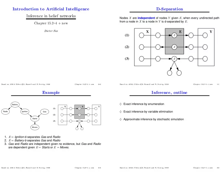
Nodes

❛

are independent of nodes

❜

given

❝

, when every undirected path from a node in

❛

to a node in

❜

is d-separated by

❝

.

X Y E (1) (2) (3)

Z Z Z

✺ ✻✼✽✾ ✿ ❀❁ ❂❃ ❁ ❄ ❅❆ ✾ ✽ ✼ ❇ ❈ ❄ ❉ ❊ ❋ ✼ ✼ ✽ ❅ ❅ ✻ ❀ ✾

• ❉❍

✿ ■ ❏ ❆ ❑ ▲ ▼ ◆ ◆❖ P ◗ ✻ ❘ ❙ ✽ ■ ▼ ❚ ❉❯ ❱ ❲ ❳ ❀ ✽❨ ▼ ❬ ▼ ❞❡ ☛ ❢ ❵ ☞ ✌

Radio Battery Ignition Gas Starts Moves X Y E (1) (2) (3)

Z Z Z

1.

❝ ❣

Ignition d-separates Gas and Radio 2.

❝ ❣

Battery d-separates Gas and Radio

• 3. Gas and Radio are independent given no evidence, but Gas and Radio

are dependent given

❝ ❣

Starts or

❝ ❣

Moves.

✺ ✻✼✽✾ ✿ ❀❁ ❂❃ ❁ ❄ ❅❆ ✾ ✽ ✼ ❇ ❈ ❄ ❉ ❊ ❋ ✼ ✼ ✽ ❅ ❅ ✻ ❀ ✾

• ❉❍

✿ ■ ❏ ❆ ❑ ▲ ▼ ◆ ◆❖ P ◗ ✻ ❘ ❙ ✽ ■ ▼ ❚ ❉❯ ❱ ❲ ❳ ❀ ✽❨ ❯ ❬ ❯ ✁❤ ✌ ✄ ✌ ✁ ✞ ✌ ✐ ☎ ✝ ✂ ☞ ✟ ✁ ✌ ❥

Exact inference by enumeration

❥

Exact inference by variable elimination

❥

Approximate inference by stochastic simulation

✺ ✻✼✽✾ ✿ ❀❁ ❂❃ ❁ ❄ ❅❆ ✾ ✽ ✼ ❇ ❈ ❄ ❉ ❊ ❋ ✼ ✼ ✽ ❅ ❅ ✻ ❀ ✾

• ❉❍

✿ ■ ❏ ❆ ❑ ▲ ▼ ◆ ◆❖ P ◗ ✻ ❘ ❙ ✽ ■ ▼ ❚ ❉❯ ❱ ❲ ❳ ❀ ✽❨ ❦ ❬ ❦

SLIDE 2

• ✁❤

✌ ✄ ✌ ✁ ✞ ✌ ❧ ♠ ✌ ✁ ✝ ❢ ✌ ✄ ☛ ✂ ✟ ☎ ✁

Slightly intelligent way to sum out variables from the joint without actually con- structing its explicit representation Simple query on the burglary network:

♥ ♦❫♣ q r ❣ st✉✈ ✇ ① ❣ st✉✈ ② ❣ ♥ ♦❫♣ ✇ r ❣ st✉✈ ✇ ① ❣ st✉✈ ②③❫④ ♦ r ❣ st✉✈ ✇ ① ❣ s t ✉ ✈ ② ❣ ⑤ ♥ ♦❫♣ ✇ r ❣ s t ✉ ✈ ✇ ① ❣ st✉✈ ② ❣ ⑤ ⑥ ⑦ ⑥ ⑧ ♥ ♦❫♣ ✇ ✈ ✇ ⑨ ✇ r ❣ st✉ ✈ ✇ ① ❣ st✉✈ ②

Rewrite full joint entries using product of CPT entries:

④ ♦❫♣ ❣ st✉ ✈ q r ❣ st✉ ✈ ✇ ① ❣ s t ✉ ✈ ② ❣ ⑤ ⑥ ⑦ ⑥ ⑧ ④ ♦❫♣ ❣ s t ✉ ✈ ② ④ ♦ ✈ ② ④ ♦ ⑨ q ♣ ❣ s t ✉ ✈ ✇ ✈ ② ④ ♦ r ❣ st✉✈ q ⑨ ② ④ ♦ ① ❣ st✉✈ q ⑨ ② ❣ ⑤ ④ ♦❫♣ ❣ st✉✈ ② ⑥ ⑦ ④ ♦ ✈ ② ⑥ ⑧ ④ ♦ ⑨ q ♣ ❣ s t ✉ ✈ ✇ ✈ ② ④ ♦ r ❣ st✉✈ q ⑨ ② ④ ♦ ① ❣ st✉✈ q ⑨ ② ✺ ✻✼✽✾ ✿ ❀❁ ❂❃ ❁ ❄ ❅❆ ✾ ✽ ✼ ❇ ❈ ❄ ❉ ❊ ❋ ✼ ✼ ✽ ❅ ❅ ✻ ❀ ✾

• ❉❍

✿ ■ ❏ ❆ ❑ ▲ ▼ ◆ ◆❖ P ◗ ✻ ❘ ❙ ✽ ■ ▼ ❚ ❉❯ ❱ ❲ ❳ ❀ ✽❨ ❲ ❬ ❲ ❞ ✁ ✝ ❢ ✌ ✄ ☛ ✂ ✟ ☎ ✁ ☛ ☞ ✍ ☎ ✄ ✟ ✂ ⑩ ❢

Exhaustive depth-first enumeration:

❶ ♦❸❷ ②

space,

❶ ♦❸❹❻❺ ②

time

❼❽ ❾ ❿➀ ➁ ➂➃➄ ➅ ❽➆ ➇ ➈

(

➉

,

➊

,

➋➌

)

➍ ➊➎➏ ➍➐ ➑

a distribution over

➉ ➒ ➐ ➓ ➏ ➎ ➑

:

➉

, the query variable

➊

, evidence specified as an event

➋ ➌

, a belief network specifying joint distribution

➔ →❸➣ ↔ ↕ ➙ ➙ ➙ ↕ ➣ ➛ ➜ ➝ → ➉ ➜ ➞

a distribution over

➉ ➟ ➠ ➍ ➊➡➢ ➤

value

➥ ➦

• f

➉ ➧ ➠

extend

➊

with value

➥ ➦

for

➉ ➝ → ➥ ➦ ➜ ➞ ❼❽ ❾ ❿➀ ➁ ➂➃ ➀ ➆ ➨ ➨

(

➩ ➂ ➁ ➇

[

➋ ➌

],

➊

)

➍ ➊ ➎ ➏ ➍➐ ➫ ➅ ➁ ❿ ➂ ➨ ➄ ➭ ➀

(

➝ → ➣ ➜

)

❼❽ ❾ ❿➀ ➁ ➂➃ ➀ ➆ ➨ ➨

(

➯➲➳➵

,

➊

)

➍ ➊➎➏ ➍➐ ➑

a real number

➒ ➟ ❼ ❿➸ ➃➺ ➻

(

➯➲ ➳➵

)

➎ ➤ ➊ ➐ ➍ ➊➎➏ ➍➐

1.0

➊ ➼ ➑ ➊ ➧ ➠ ➽ ➞ ➾ ➄ ➁ ➇ ➃

(

➯➲ ➳ ➵

)

➒ ➟ ➽

has value

➚

in

➊ ➎ ➤ ➊ ➐ ➍ ➊ ➎ ➏ ➍ ➐ ➪ → ➶ ➹ ➪ ➘ →❸➴ ➜ ➜❸➷ ❼❽ ❾ ❿ ➀ ➁ ➂➃ ➀ ➆ ➨ ➨

(

➬ ➀ ➇ ➃

(

➯➲ ➳ ➵

),

➊

)

➊ ➼ ➑ ➊ ➍ ➊➎➏ ➍ ➐ ➮ ➱ ➪ → ➶ ➹ ➪ ➘ →❸➴ ➜ ➜❸➷ ❼❽ ❾ ❿ ➀ ➁ ➂➃ ➀ ➆ ➨ ➨

(

➬ ➀ ➇ ➃

(

➯➲➳➵

),

➊ ➱

) where

➊ ➱

is

➊

extended with

➴ ✃ ➶ ✺ ✻✼✽✾ ✿ ❀❁ ❂❃ ❁ ❄ ❅❆ ✾ ✽ ✼ ❇ ❈ ❄ ❉ ❊ ❋ ✼ ✼ ✽ ❅ ❅ ✻ ❀ ✾

• ❉❍

✿ ■ ❏ ❆ ❑ ▲ ▼ ◆ ◆❖ P ◗ ✻ ❘ ❙ ✽ ■ ▼ ❚ ❉❯ ❱ ❲ ❳ ❀ ✽❨ ❚ ❬ ❚ ✁❤ ✌ ✄ ✌ ✁ ✞ ✌ ❧ ♠❒❐ ☛ ✄ ✟ ☛ ❧ ☞ ✌ ✌ ☞ ✟ ❢ ✟ ✁ ☛ ✂ ✟ ☎ ✁

Enumeration is inefficient: repeated computation e.g., computes

④ ♦ r ❣ st✉ ✈ q ⑨ ② ④ ♦ ① ❣ st✉✈ q ⑨ ②

for each value of

✈

Variable elimination: carry out summations right-to-left, storing intermediate results (factors) to avoid recomputation

♥ ♦❫♣ q r ❣ st✉✈ ✇ ① ❣ st✉✈ ② ❣ ⑤ ♥ ♦❫♣ ② ❮ ❰Ï Ð Ñ ⑥ ⑦ ④ ♦ ✈ ② ❮ ❰ Ï Ð Ò ⑥ ⑧ ♥ ♦ ⑨ q ♣ ✇ ✈ ② ❮ ❰ Ï Ð Ó ④ ♦ r ❣ st✉✈ q ⑨ ② ❮ ❰ Ï Ð Ô ④ ♦ ① ❣ st✉ ✈ q ⑨ ② ❮ ❰Ï Ð Õ ❣ ⑤ ♥ ♦❫♣ ② ⑥ ⑦ ④ ♦ ✈ ② ⑥ ⑧ ♥ ♦ ⑨ q ♣ ✇ ✈ ② ④ ♦ r ❣ st✉✈ q ⑨ ② Ö Õ ♦ ⑨ ② ❣ ⑤ ♥ ♦❫♣ ② ⑥ ⑦ ④ ♦ ✈ ② ⑥ ⑧ ♥ ♦ ⑨ q ♣ ✇ ✈ ② Ö Ô ♦ ⑨ ② Ö Õ ♦ ⑨ ② ❣ ⑤ ♥ ♦❫♣ ② ⑥ ⑦ ④ ♦ ✈ ② ⑥ ⑧ Ö Ó ♦ ⑨ ✇ × ✇ ✈ ② Ö Ô ♦ ⑨ ② Ö Õ ♦ ⑨ ② ❣ ⑤ ♥ ♦❫♣ ② ⑥ ⑦ ④ ♦ ✈ ② ÖÙØ Ó Ô Õ ♦ × ✇ ✈ ②

(sum out

Ú

)

❣ ⑤ ♥ ♦❫♣ ② Ö Ø Ò Ø Ó Ô Õ ♦ × ②

(sum out

❝

)

❣ ⑤ Ö Ñ ♦ × ②ÜÛ Ö Ø Ò Ø Ó Ô Õ ♦ × ② ✺ ✻✼✽✾ ✿ ❀❁ ❂❃ ❁ ❄ ❅❆ ✾ ✽ ✼ ❇ ❈ ❄ ❉ ❊ ❋ ✼ ✼ ✽ ❅ ❅ ✻ ❀ ✾

• ❉❍

✿ ■ ❏ ❆ ❑ ▲ ▼ ◆ ◆❖ P ◗ ✻ ❘ ❙ ✽ ■ ▼ ❚ ❉❯ ❱ ❲ ❳ ❀ ✽❨ Ý ❬ Ý Þ ☎ ❢ ❵ ☞ ✌ ❡ ✟ ✂ ♠ ☎ ❤ ✌ ❡ ☛ ✞ ✂ ✟ ✁❤ ✌ ✄ ✌ ✁ ✞ ✌

Singly connected networks (or polytrees): – any two nodes are connected by at most one (undirected) path – time and space cost of variable elimination are

❶ ♦❸❹❻ß ❷ ②

Multiply connected networks: – can reduce 3SAT to exact inference

à

NP-hard – equivalent to counting 3SAT models

à

#P-complete

✺ ✻✼✽✾ ✿ ❀❁ ❂❃ ❁ ❄ ❅❆ ✾ ✽ ✼ ❇ ❈ ❄ ❉ ❊ ❋ ✼ ✼ ✽ ❅ ❅ ✻ ❀ ✾

• ❉❍

✿ ■ ❏ ❆ ❑ ▲ ▼ ◆ ◆❖ P ◗ ✻ ❘ ❙ ✽ ■ ▼ ❚ ❉❯ ❱ ❲ ❳ ❀ ✽❨ á ❬ á

SLIDE 3 ✁❤ ✌ ✄ ✌ ✁ ✞ ✌ ❧ ♠❒â ✂ ☎ ✞ ⑩ ☛ â ✂ ✟ ✞ â ✟ ❢ ✝ ☞ ☛ ✂ ✟ ☎ ✁

Basic idea: 1) Draw

ã

samples from a sampling distribution

ä

2) Compute an approximate posterior probability

å ④

3) Show this converges to the true probability

④

Outline: – Sampling from an empty network – Rejection sampling: reject samples disagreeing with evidence – Likelihood weighting: use evidence to weight samples – MCMC: sample from a stochastic process whose stationary distribution is the true posterior

✺ ✻✼✽✾ ✿ ❀❁ ❂❃ ❁ ❄ ❅❆ ✾ ✽ ✼ ❇ ❈ ❄ ❉ ❊ ❋ ✼ ✼ ✽ ❅ ❅ ✻ ❀ ✾

• ❉❍

✿ ■ ❏ ❆ ❑ ▲ ▼ ◆ ◆❖ P ◗ ✻ ❘ ❙ ✽ ■ ▼ ❚ ❉❯ ❱ ❲ ❳ ❀ ✽❨ ❖ ❬ ❖ ❴ ☛ ❢ ❵ ☞ ✟ ✁ ✍ ❤ ✄ ☎ ❢ ☛ ✁ ✌ ❢ ❵ ✂ ♠ ✁ ✌ ✂æ ☎ ✄ç ➟ ➏ ➐ ➢ ➎ ➒ ➠ ➐ è ➁ ➄ ➅ ➁é ➂ ❿ ➸ ➨ ➀

(

➋ ➌

)

➍ ➊➎➏ ➍➐ ➑

an event sampled from

➔ →❸➣ ↔ ↕ ➙ ➙ ➙ ↕ ➣ ➛ ➜

specified b

ê ➞

an event with

ë

elements

➟ ➠ ➍ ì ✃ í ➎ ➠ ë ➧ ➠ ➥ ➦ ➞

a random sample from

➔ → ➣ ➦ ➹ ➪ ➘îï ëðñ → ➣ ➦ ➜ ➜ ➍ ➊ ➎ ➏ ➍➐ ê ♥ ♦ ò óô ✉ ❹ õ ② ❣ ö ÷ ø ù ✇ ÷ ø ù ú

sample

û st✉ ✈ ♥ ♦ ä ü tý ❷þ ó ✈ t q ò ó ô ✉ ❹ õ ② ❣ ö ÷ øÿ ✇ ÷ ø

• ú

sample

û Ö ⑨ ó ✁ ✈ ♥ ♦ ✂ ⑨ ý ❷ q ò ó ô ✉ ❹ õ ② ❣ ö ÷ ø ✄ ✇ ÷ ø ☎ ú

sample

û st✉ ✈ ♥ ♦ ✆ ✈ s ✝ t ⑨ ✁ ✁ q✟✞ ä ü tý ❷ þ ó ✈ t ✇ ✂ ⑨ ý ❷ ② ❣ ö ÷ ø

• ✇

÷ ø ÿ ú

sample

û st✉ ✈

P(C) = .5 C T F C P(S) T F .10 .50 S R P(W) T T T F F T F F .90 .90 .00 .99 Cloudy Rain Sprinkler Wet Grass

✺ ✻✼✽✾ ✿ ❀❁ ❂❃ ❁ ❄ ❅❆ ✾ ✽ ✼ ❇ ❈ ❄ ❉ ❊ ❋ ✼ ✼ ✽ ❅ ❅ ✻ ❀ ✾

• ❉❍

✿ ■ ❏ ❆ ❑ ▲ ▼ ◆ ◆❖ P ◗ ✻ ❘ ❙ ✽ ■ ▼ ❚ ❉❯ ❱ ❲ ❳ ❀ ✽❨ ◆ ❬ ◆ ❴ ☛ ❢ ❵ ☞ ✟ ✁ ✍ ❤ ✄ ☎ ❢ ☛ ✁ ✌ ❢ ❵ ✂ ♠ ✁ ✌ ✂æ ☎ ✄ç ✞ ☎ ✁ ✂ ✆ ✠

Probability that

✡ ☛ ☞ ✌ ☛ ✍ ✎✏ ✑✒✓

generates a particular event

ä ✔ ✕ ♦✗✖ ✘ ø ø ø ✖ ❺ ② ❣ ✙ ❺ ✚ ✛ ✘ ④ ♦ ✖ ✚ q ④ ⑨ t ✈ ❷ s ✁ ♦ ❛ ✚ ② ② ❣ ④ ♦✗✖ ✘ ø ø ø ✖ ❺ ②

i.e., the true prior probability Let

ã ✔ ✕ ♦✢✜ ❣ ✣ ②

be the number of samples generated for which

✜ ❣ ✣

, for any set of variables

✜

. Then

å ④ ♦✢✜ ❣ ✣ ② ❣ ã ✔ ✕ ♦✢✜ ❣ ✣ ② ③ ã

and

✤✥✦ ✧ ★ ✩ å ④ ♦✢✜ ❣ ✣ ② ❣ ✪ ✫ ä ✔ ✕ ♦✢✜ ❣ ✣ ✇ ✬ ❣ ✭ ② ❣ ✪ ✫ ④ ♦✢✜ ❣ ✣ ✇ ✬ ❣ ✭ ② ❣ ④ ♦✢✜ ❣ ✣ ②

That is, estimates derived from

✡ ☛ ☞ ✌ ☛ ✍ ✎✏ ✑✒✓

are consistent

✺ ✻✼✽✾ ✿ ❀❁ ❂❃ ❁ ❄ ❅❆ ✾ ✽ ✼ ❇ ❈ ❄ ❉ ❊ ❋ ✼ ✼ ✽ ❅ ❅ ✻ ❀ ✾

• ❉❍

✿ ■ ❏ ❆ ❑ ▲ ▼ ◆ ◆❖ P ◗ ✻ ❘ ❙ ✽ ■ ▼ ❚ ❉❯ ❱ ❲ ❳ ❀ ✽ ❨ ▼ ❩ ❬ ▼ ❩ ✮ ✌ ✯ ✌ ✞ ✂ ✟ ☎ ✁ â ☛ ❢ ❵ ☞ ✟ ✁ ✍ å ♥ ♦ ❛ q✱✰ ②

estimated from samples agreeing with

✰ ➟ ➏ ➐ ➢ ➎ ➒ ➠ ➐ ➬ ➀ ✲ ➀ ✳ ➃➄ ➅ ❽ é ➂ ❿ ➸ ➨ ➄ ❽ ✴

(

➉

,

➊

,

➋ ➌

,

✵

)

➍ ➊ ➎ ➏ ➍➐ ➑

an approximation to

➪ → ➣ ➹ ➊ ➜ ✶

[

➉

]

➞

a vector of counts over

➉

, initially zero

➟ ➠ ➍ ✷

= 1 to

✸ ➧ ➠ ê ➞ è ➁ ➄ ➅ ➁ é ➂ ❿ ➸ ➨ ➀

(

➋ ➌

)

➒ ➟ ê

is consistent with

➊ ➎ ➤ ➊ ➐ ✶

[

✹

]

➞ ✶

[

✹

]+1 where

✹

is the value of

➉

in

ê ➍ ➊ ➎ ➏ ➍➐ ➫ ➅ ➁ ❿ ➂ ➨ ➄ ➭ ➀

(

✶

[

➉

])

E.g., estimate

♥ ♦ ✂ ⑨ ý ❷ q ä ü tý ❷þ ó ✈ t ❣ st✉✈ ②

using 100 samples 27 samples have

ä ü tý ❷ þ ó ✈ t ❣ st✉✈

Of these, 8 have

✂ ⑨ ý ❷ ❣ s t ✉ ✈

and 19 have

✂ ⑨ ý ❷ ❣ Ö ⑨ ó ✁ ✈

.

å ♥ ♦ ✂ ⑨ ý ❷ q ä ü tý ❷ þ ó✈ t ❣ st✉ ✈ ② ❣ ✺ ✌ ☛ ✏ ✎ ✒ ☞✻ ✓ ♦ ö ✄ ✇ ÿ

• ú

② ❣ ö ÷ ø ☎ ✼ ✇ ÷ ø ✽ ÷ ✾ ú

Similar to a basic real-world empirical estimation procedure

✺ ✻✼✽✾ ✿ ❀❁ ❂❃ ❁ ❄ ❅❆ ✾ ✽ ✼ ❇ ❈ ❄ ❉ ❊ ❋ ✼ ✼ ✽ ❅ ❅ ✻ ❀ ✾

• ❉❍

✿ ■ ❏ ❆ ❑ ▲ ▼ ◆ ◆❖ P ◗ ✻ ❘ ❙ ✽ ■ ▼ ❚ ❉❯ ❱ ❲ ❳ ❀ ✽ ❨ ▼ ▼ ❬ ▼ ▼

SLIDE 4 ✠ ✁ ☛ ☞ ♠ â ✟ â ☎ ❤ ✄ ✌ ✯ ✌ ✞ ✂ ✟ ☎ ✁ â ☛ ❢ ❵ ☞ ✟ ✁ ✍ å ♥ ♦ ❛ q✱✰ ② ❣ ⑤ ✿ ✔ ✕ ♦ ❛ ✇ ✰ ②

(algorithm defn.)

❣ ✿ ✔ ✕ ♦ ❛ ✇ ✰ ② ③ ã ✔ ✕ ♦ ✰ ②

(normalized by

ã ✔ ✕ ♦ ✰ ②

)

❀ ♥ ♦ ❛ ✇ ✰ ② ③❫④ ♦ ✰ ②

(property of

✡ ☛ ☞ ✌ ☛ ✍ ✎✏ ✑✒✓

)

❣ ♥ ♦ ❛ q✱✰ ②

(defn. of conditional probability) Hence rejection sampling returns consistent posterior estimates Problem: hopelessly expensive if

④ ♦ ✰ ②

is small

✺ ✻✼✽✾ ✿ ❀❁ ❂❃ ❁ ❄ ❅❆ ✾ ✽ ✼ ❇ ❈ ❄ ❉ ❊ ❋ ✼ ✼ ✽ ❅ ❅ ✻ ❀ ✾

• ❉❍

✿ ■ ❏ ❆ ❑ ▲ ▼ ◆ ◆❖ P ◗ ✻ ❘ ❙ ✽ ■ ▼ ❚ ❉❯ ❱ ❲ ❳ ❀ ✽ ❨ ▼ ❯ ❬ ▼ ❯ ❁ ✟ ç ✌ ☞ ✟ ⑩ ☎ ☎ ✆ æ ✌ ✟ ✍ ⑩ ✂ ✟ ✁ ✍

Idea: fix evidence variables, sample only nonevidence variables, and weight each sample by the likelihood it accords the evidence

➟ ➏ ➐ ➢ ➎ ➒ ➠ ➐ ❂ ➀ ➄ ✴ ❃ ➃ ➀❄ é ➂ ❿ ➸ ➨ ➀

(

➋ ➌

,

➊

)

➍ ➊ ➎ ➏ ➍➐ ➑

an event and a weight

ê ➞

an event with

ë

elements;

❅ ➞

1

➟ ➠ ➍ ❆

= 1

➎ ➠ ë ➧ ➠ ➒ ➟ ➣ ➦

has a value

➥ ➦

in

➊ ➎ ➤ ➊ ➐ ❅ ➞ ❅ ➷ ➪ → ➣ ➦ ✃ ➥ ➦ ➹ ➪ ➘îï ëð ñ → ➣ ➦ ➜ ➜ ➊ ➼ ➑ ➊ ➥ ➦ ➞

a random sample from

➔ → ➣ ➦ ➹ ➪ ➘ î ï ë ð ñ → ➣ ➦ ➜ ➜ ➍ ➊ ➎ ➏ ➍➐ ê

,

❅ ➟ ➏ ➐ ➢ ➎ ➒ ➠ ➐ ❇ ➄ ➈ ➀ ➨ ➄ ❃ ➅ ➅ ❄ ❂ ➀ ➄ ✴ ❃ ➃ ➄ ❽ ✴

(

➉

,

➊

,

➋ ➌

,

✵

)

➍ ➊➎➏ ➍➐ ➑

an approximation to

➪ → ➣ ➹ ➊ ➜ ❈ ❉ ➉ ❊ ➞

a vector of weighted counts over

➉

, initially zero

➟ ➠ ➍ ✷

= 1 to

✸ ➧ ➠ ê

,

❅ ➞ ❂ ➀ ➄ ✴ ❃ ➃ ➀❄ é ➂ ❿ ➸ ➨ ➀

(

➋➌

)

❈ ❉ ✹ ❊ ➞ ❈ ❉ ✹ ❊ ❋ ❅

where

✹

is the value of

➉

in

ê ➍ ➊ ➎ ➏ ➍➐ ➫ ➅ ➁ ❿ ➂ ➨ ➄ ➭ ➀

(

❈ ❉ ➉ ❊

)

✺ ✻✼✽✾ ✿ ❀❁ ❂❃ ❁ ❄ ❅❆ ✾ ✽ ✼ ❇ ❈ ❄ ❉ ❊ ❋ ✼ ✼ ✽ ❅ ❅ ✻ ❀ ✾

• ❉❍

✿ ■ ❏ ❆ ❑ ▲ ▼ ◆ ◆❖ P ◗ ✻ ❘ ❙ ✽ ■ ▼ ❚ ❉❯ ❱ ❲ ❳ ❀ ✽ ❨ ▼ ❦ ❬ ▼ ❦ ❁ ✟ ç ✌ ☞ ✟ ⑩ ☎ ☎ ✆ æ ✌ ✟ ✍ ⑩ ✂ ✟ ✁ ✍ ✌ ❡ ☛ ❢ ❵ ☞ ✌

Estimate

♥ ♦ ✂ ⑨ ý ❷ q ä ü t ý ❷ þ ó✈ t ❣ st✉✈ ✇ ✆ ✈ s ✝ t ⑨ ✁ ✁ ❣ st✉✈ ②

P(C) = .5 C P(R) T F .80 .20 C P(S) T F .10 .50 S R P(W) T T T F F T F F .90 .90 .00 .99 Cloudy Rain Sprinkler Wet Grass

true true

✺ ✻✼✽✾ ✿ ❀❁ ❂❃ ❁ ❄ ❅❆ ✾ ✽ ✼ ❇ ❈ ❄ ❉ ❊ ❋ ✼ ✼ ✽ ❅ ❅ ✻ ❀ ✾

• ❉❍

✿ ■ ❏ ❆ ❑ ▲ ▼ ◆ ◆❖ P ◗ ✻ ❘ ❙ ✽ ■ ▼ ❚ ❉❯ ❱ ❲ ❳ ❀ ✽ ❨ ▼ ❲ ❬ ▼ ❲ ❁

• ✌

❡ ☛ ❢ ❵ ☞ ✌ ✞ ☎ ✁ ✂ ✆ ✠

Sample generation process: 1.

❍■ ÿ ø ÷

• 2. Sample

♥ ♦ ò ó ô ✉ ❹ õ ② ❣ ö ÷ ø ù ✇ ÷ ø ù ú

; say

st✉✈

3.

ä ü t ý ❷ þ ó✈ t

has value

st✉✈

, so

❍■ ❍ Û ④ ♦ ä ü tý ❷ þ ó ✈ t ❣ s t ✉ ✈ q ò óô ✉ ❹ õ ❣ s t ✉ ✈ ② ❣ ÷ øÿ

• 4. Sample

♥ ♦ ✂ ⑨ ý ❷ q ò óô ✉ ❹ õ ❣ s t ✉ ✈ ② ❣ ö ÷ ø ✄ ✇ ÷ ø ☎ ú

; say

st✉✈

5.

✆ ✈ s ✝ t ⑨ ✁ ✁

has value

st✉✈

, so

❍■ ❍ Û ④ ♦ ✆ ✈ s ✝ t ⑨ ✁ ✁ ❣ s t ✉ ✈ q ä ü tý ❷þ ó ✈ t ❣ st✉✈ ✇ ✂ ⑨ ý ❷ ❣ st✉✈ ② ❣ ÷ ø ÷

• ✺

✻✼✽✾ ✿ ❀❁ ❂❃ ❁ ❄ ❅❆ ✾ ✽ ✼ ❇ ❈ ❄ ❉ ❊ ❋ ✼ ✼ ✽ ❅ ❅ ✻ ❀ ✾

• ❉❍

✿ ■ ❏ ❆ ❑ ▲ ▼ ◆ ◆❖ P ◗ ✻ ❘ ❙ ✽ ■ ▼ ❚ ❉❯ ❱ ❲ ❳ ❀ ✽ ❨ ▼ ❚ ❬ ▼ ❚

SLIDE 5 ✠ ❵ ❵ ✄ ☎ ❡ ✟ ❢ ☛ ✂✌ ✟ ✁❤ ✌ ✄ ✌ ✁ ✞ ✌ ✝ â ✟ ✁ ✍❑❏ Þ ❏ Þ

“State” of network = current assignment to all variables Generate next state by sampling one variable given its Markov blanket Sample each variable in turn, keeping evidence fixed Approaches stationary distribution: long-run fraction of time spent in each state is exactly proportional to its posterior probability Main computational problems: 1) Difficult to tell if convergence has been achieved 2) Can be wasteful if Markov blanket is large:

④ ♦ ❜ ✚ q ① ♣ ♦ ❜ ✚ ② ②

won’t change much (law of large numbers)

✺ ✻✼✽✾ ✿ ❀❁ ❂❃ ❁ ❄ ❅❆ ✾ ✽ ✼ ❇ ❈ ❄ ❉ ❊ ❋ ✼ ✼ ✽ ❅ ❅ ✻ ❀ ✾

• ❉❍

✿ ■ ❏ ❆ ❑ ▲ ▼ ◆ ◆❖ P ◗ ✻ ❘ ❙ ✽ ■ ▼ ❚ ❉❯ ❱ ❲ ❳ ❀ ✽ ❨ ▼ Ý ❬ ▼ Ý ▲ ✌ ✄ ❤ ☎ ✄ ❢ ☛ ✁ ✞ ✌ ☎ ❤ ☛ ❵ ❵ ✄ ☎ ❡ ✟ ❢ ☛ ✂ ✟ ☎ ✁ ☛ ☞ ✍ ☎ ✄ ✟ ✂ ⑩ ❢ â

Absolute approximation:

q ④ ♦ ❛ q ✰ ②◆▼ å ④ ♦ ❛ q✱✰ ② q ❖ P

Relative approximation:

◗ ✔ ❘ ❙ ◗ ✰ ❚✟❯❲❱ ✔ ❘ ❙ ◗ ✰ ❚ ◗ ✔ ❘ ❙ ◗ ✰ ❚ ❖ P

Relative

à

absolute since

÷ ❖ ④ ❖ ÿ

Randomized algorithms may fail with probability at most

❳

Polytime approximation: poly

♦❸❷ ✇ P ❯ ✘ ✇ ✤ ❨ ❩ ❳ ❯ ✘ ②

Theorem (Dagum and Luby, 1993): both absolute and relative approximation for either deterministic or randomized algorithms are NP-hard for any

P ✇ ❳ ❬ ÷ ø ù ✺ ✻✼✽✾ ✿ ❀❁ ❂❃ ❁ ❄ ❅❆ ✾ ✽ ✼ ❇ ❈ ❄ ❉ ❊ ❋ ✼ ✼ ✽ ❅ ❅ ✻ ❀ ✾

• ❉❍

✿ ■ ❏ ❆ ❑ ▲ ▼ ◆ ◆❖ P ◗ ✻ ❘ ❙ ✽ ■ ▼ ❚ ❉❯ ❱ ❲ ❳ ❀ ✽ ❨ ▼ á ❬ ▼ á Þ ☛ â ✌ â ✂ ✝ ✆ ♠❑❭ ▲ ☛ ✂ ⑩ ✡ ✁ ✆ ✌ ✄

• ❪

Diagnostic expert system for lymph-node diseases. Deciding on vocabulary: 8 hours Design topology of network: 35 hours Make 14,000 probability assessments: 40 hours Pathfinder now outperforms experts who were consulted during its creation!

✺ ✻✼✽✾ ✿ ❀❁ ❂❃ ❁ ❄ ❅❆ ✾ ✽ ✼ ❇ ❈ ❄ ❉ ❊ ❋ ✼ ✼ ✽ ❅ ❅ ✻ ❀ ✾

• ❉❍

✿ ■ ❏ ❆ ❑ ▲ ▼ ◆ ◆❖ P ◗ ✻ ❘ ❙ ✽ ■ ▼ ❚ ❉❯ ❱ ❲ ❳ ❀ ✽ ❨ ▼ ❖ ❬ ▼ ❖