Overview Announcements: Homework 1 due today Homework 2 will be - - PowerPoint PPT Presentation

CMPSCI 370: Intro to Computer Vision

Image processing

[ quantization, color maps, image enhancement ] University of Massachusetts, Amherst February 9, 2016 Instructor: Subhransu Maji

Slides credit: Erik Learned-Miller and others

• Announcements:
• Homework 1 due today
• Homework 2 will be posted soon
• Honors section will meet today at 4pm
• Today’s lecture:
• Review color constancy
• Image processing
• signal quantization
• color representation
• enhancing images intro

Overview

2

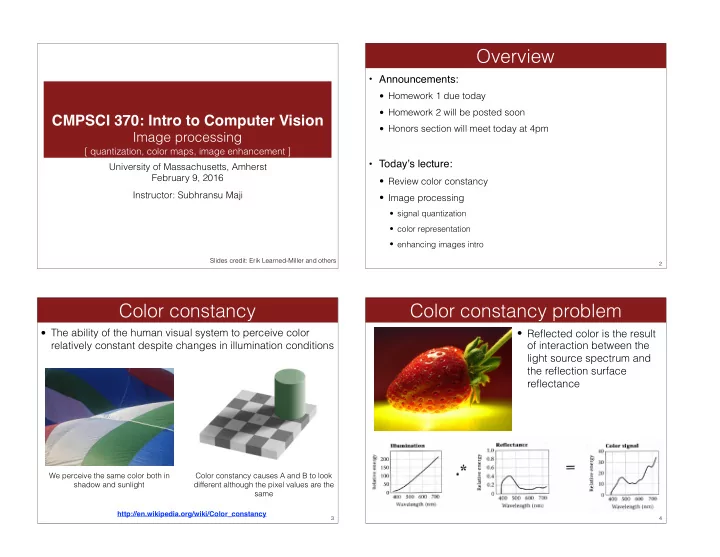
• The ability of the human visual system to perceive color

relatively constant despite changes in illumination conditions

Color constancy

3

Color constancy causes A and B to look different although the pixel values are the same We perceive the same color both in shadow and sunlight

http://en.wikipedia.org/wiki/Color_constancy

Color constancy problem

4

• Reflected color is the result
• f interaction between the

light source spectrum and the reflection surface reflectance

Color constancy

5

Color constancy causes A and B to look different although the pixel values are the same

Mathematically we have a x b = c; Given c we want to recover a and b.

x

light paint

Color constancy

6

#1 white and gold

• r

#2 blue and black # 1 light is blue so white is tinted blue and gold doesn’t really change # 2 light is yellow, so black reflects the yellow and the blue is unaffected

Color constancy

7

http://xkcd.com/1492/

Color constancy

8

http://xkcd.com/1492/

• The visual system changes its sensitivity depending on the

luminances prevailing in the visual field

• The exact mechanism is poorly understood
• Adapting to different brightness levels
• Changing the size of the iris opening (i.e., the aperture) changes the

amount of light that can enter the eye

• Think of walking into a building from full sunshine
• Adapting to different color temperature
• The receptive cells on the retina change their sensitivity
• For example: if there is an increased amount of red light, the cells

receptive to red decrease their sensitivity until the scene looks white again

• We actually adapt better in brighter scenes: This is why candlelit scenes

still look yellow

Chromatic adaptation

9

http://www.schorsch.com/kbase/glossary/adaptation.html

• When looking at a picture on screen or print, our eyes are

adapted to the illuminant of the room, not to that of the scene in the picture

• When the white balance is not correct, the picture will have an

unnatural color “cast”

White balance

10

http://www.cambridgeincolour.com/tutorials/white-balance.htm incorrect white balance correct white balance

• Film cameras:
• Different types of film or different filters for different illumination conditions
• Digital cameras:
• Automatic white balance
• White balance settings corresponding to 


several common illuminants

• Custom white balance using a reference 

• bject

White balance

11

http://www.cambridgeincolour.com/tutorials/white-balance.htm

• Von Kries adaptation
• Multiply each channel by a gain factor
• Best way: gray card
• Take a picture of a neutral object (white or gray)
• Deduce the weight of each channel
• If the object is recoded as rw, gw, bw use weights 1/rw, 1/gw, 1/bw

White balance

12 Source: L. Lazebnik

• Without gray cards: we need to “guess” which pixels

correspond to white objects

• Gray world assumption
• The image average rave, gave, bave is gray
• Use weights 1/rave, 1/gave, 1/bave
• Brightest pixel assumption
• Highlights usually have the color of the light source
• Use weights inversely proportional to the values of the brightest pixels
• Gamut mapping
• Gamut: convex hull of all pixel colors in an image
• Find the transformation that matches the gamut of the image to the gamut
• f a “typical” image under white light
• Use image statistics, learning techniques

White balance

13 Source: L. Lazebnik

Image formation

14

• What is an image before you digitize it?
• Continuous range of wavelengths
• 2-dimensional extent
• Continuous range of power at each point

Pre-digitization image

15

• To simplify, consider only a brightness image
• Two-dimensional (continuous range of locations)
• Continuous range of brightness values
• This is equivalent to a two-dimensional function over a

plane

Brightness images

16

An image as a surface

17

How do we represent this continuous two dimensional surface efficiently?

• Sampling strategies
• Spatial sampling
• How many pixels?
• What arrangement of pixels?
• Brightness sampling
• How many brightness values?
• Spacing of brightness values?
• For video, also the question of time sampling.

Discretization

18

• Goal: determine a mapping from a continuous signal (e.g.

analog video signal) to one of K discrete (digital) levels.

Signal quantization

19

• I(x,y) = continuous signal: 0 ≤ I ≤ M
• Want to quantize to K values 0,1,....K-1
• K usually chosen to be a power of 2:
• Mapping from input signal to output signal is to be determined.
• Several types of mappings: uniform, logarithmic, etc.

Quantization

20

K: #Levels #Bits 2 1 4 2 8 3 16 4 32 5 64 6 128 7 256 8

Choice of K

21

Choice of K

22

False contours problem

23

“Dithering” adds random noise to reduce false contours 16 colors with random noise

https://en.wikipedia.org/wiki/Dither

• riginal image
• Uniform sampling divides the signal range [0-M] into K

equal-sized intervals.

• The integers 0,...K-1 are assigned to these intervals.
• All signal values within an interval are represented by the

associated integer value.

• Defines a mapping:

Choice of the function: uniform

24

• Signal is: log I(x,y)
• Effect is:
• Detail enhanced in the low signal values at expense of detail

in high signal values.

Logarithmic quantization

25

Logarithmic quantization

26

• Given a 24 bit color image (8 bits for R, G, B)
• Turn on 3 subpixels with power proportional to RGB values

Color displays

27

https://en.wikipedia.org/wiki/File:Pixel_geometry_01_Pengo.jpg

A single pixel.

“White” text on color display

28

http://en.wikipedia.org/wiki/Subpixel_rendering

• 8 bit image: 256 different values.
• Simplest way to display: map each number to a gray value:
• 0 g (0.0, 0.0, 0.0) or (0,0,0)
• 1 g (0.0039, 0.0039, 0.0039) or (1,1,1)
• 2 g (0.0078, 0.0078, 0.0078) or (2,2,2)
• ...
• 255 g (1.0, 1.0, 1.0) or (255,255,255)
• This is called a grayscale mapping.

Lookup tables

29

Lookup tables

30

• We can also use other mappings:
• 0 g (17, 25, 89)
• 1 g (45, 32, 200)
• ...
• 255 g (233,1,4)
• These are called lookup tables.

Non-gray lookup tables

31

More colormaps

32

colormap jet; colormap winter;

Fun with Matlab

33

• What can we do to “enhance” an image after it has already

been digitized?

• We can make the information that is there easier to visualize.
• We can guess at data that is not there, but we cannot be sure, in

general.

Enhancing images

34

contrast enhancement deblurring

• Two methods:
• Normalize the data (contrast stretching)
• Transform the data (histogram equalization)

Contrast enhancement

35

Contrast stretching

36

histogram before after

image source: wikipedia map this to 255 map this to 0

• Basic idea: scale the brightness range of the image to
• ccupy the full range of values
• Issues:
• What happens if there is one bright pixel?
• What happens if there is one dark pixel?

Contrast stretching

37

I ← floor ✓ I − min(I) max(I) − min(I) × 255 ◆

map this to 0 map this to 255

• imcontrast() — contrast stretching

Matlab demo

38

Histogram equalization

39

histogram before after

make the distribution close to the uniform distribution