
– 1 – CS:APP3e
Computer Architecture: Pipelining
CSci 2021: Machine Architecture and Organization March 25th-27th, 2020 Your instructor: Stephen McCamant Based on slides originally by: Randy Bryant and Dave O’Hallaron
– 2 – CS:APP3e
Overview
General Principles of Pipelining
Goal Difficulties
Creating a Pipelined Y86-64 Processor
Rearranging SEQ Inserting pipeline registers Problems with data and control hazards – 3 – CS:APP3e
Real-World Pipelines: Car Washes
Idea
Divide process into
independent stages
Move objects through stages
in sequence
At any given times, multiple
- bjects being processed
Sequential Parallel Pipelined
– 4 – CS:APP3e
Computational Example
System
Computation requires total of 300 picoseconds Additional 20 picoseconds to save result in register Must have clock cycle of at least 320 ps Combinational logic R e g 300 ps 20 ps Clock Delay = 320 ps Throughput = 3.12 GIPS – 5 – CS:APP3e
3-Way Pipelined Version
System
Divide combinational logic into 3 blocks of 100 ps each Can begin new operation as soon as previous one passes
through stage A.
Begin new operation every 120 ps Overall latency increases 360 ps from start to finish R e g Clock Comb. logic A R e g Comb. logic B R e g Comb. logic C 100 ps 20 ps 100 ps 20 ps 100 ps 20 ps Delay = 360 ps Throughput = 8.33 GIPS
– 6 – CS:APP3e
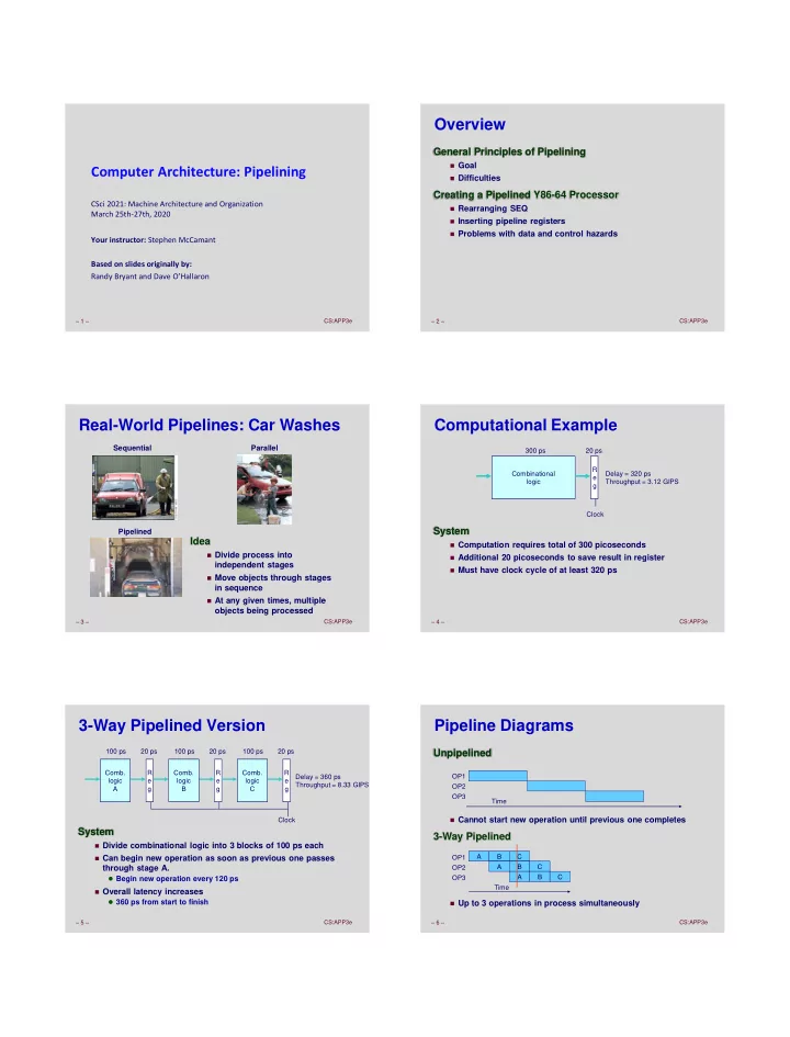
Pipeline Diagrams
Unpipelined
Cannot start new operation until previous one completes
3-Way Pipelined
Up to 3 operations in process simultaneously Time OP1 OP2 OP3 Time A B C A B C A B C OP1 OP2 OP3