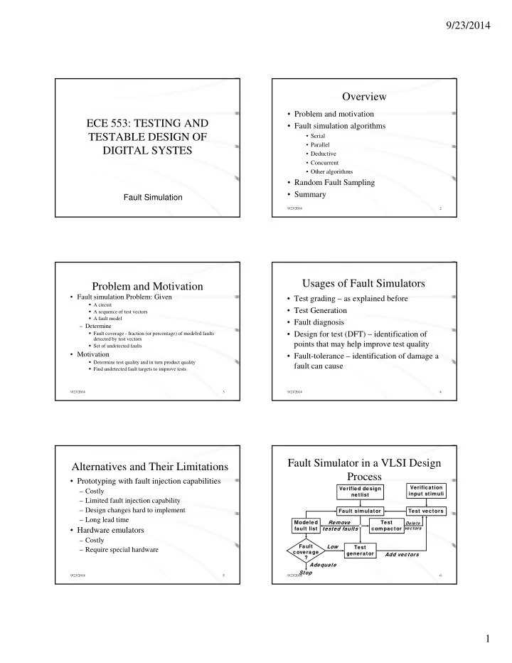
Overview Problem and motivation ECE 553: TESTING AND Fault - - PDF document

9/23/2014 1

ECE 553: TESTING AND TESTABLE DESIGN OF DIGITAL SYSTES DIGITAL SYSTES

Fault Simulation

Overview

• Problem and motivation
• Fault simulation algorithms
• Serial
• Parallel

9/23/2014 2

• Deductive
• Concurrent
• Other algorithms
• Random Fault Sampling
• Summary

Problem and Motivation

• Fault simulation Problem: Given
• A circuit
• A sequence of test vectors
• A fault model

– Determine

9/23/2014 3

• Fault coverage - fraction (or percentage) of modeled faults

detected by test vectors

• Set of undetected faults
• Motivation
• Determine test quality and in turn product quality
• Find undetected fault targets to improve tests

Usages of Fault Simulators

• Test grading – as explained before
• Test Generation
• Fault diagnosis

D i f (DFT) id ifi i f

9/23/2014 4

• Design for test (DFT) – identification of

points that may help improve test quality

• Fault-tolerance – identification of damage a

fault can cause

Alternatives and Their Limitations

• Prototyping with fault injection capabilities

– Costly – Limited fault injection capability – Design changes hard to implement

9/23/2014 5

– Long lead time

• Hardware emulators

– Costly – Require special hardware

Fault Simulator in a VLSI Design Process

Verified design netlist Verification input stimuli Fault simulator Test vectors

9/23/2014 6

Modeled fault list Test generator Test compactor Fault coverage ? Remove tested faults

Delete vectors

Add vectors Low Adequate Stop

9/23/2014 2

Fault Simulation Scenario

• Circuit model: mixed-level
• Mostly logic with some switch-level for high-impedance

(Z) and bidirectional signals

• High-level models (memory, etc.) with pin faults
• Signal states: logic

9/23/2014 7

g g

• Two (0, 1) or three (0, 1, X) states for purely Boolean

logic circuits

• Four states (0, 1, X, Z) for sequential MOS circuits
• Timing:
• Zero-delay for combinational and synchronous circuits
• Mostly unit-delay for circuits with feedback

Fault Simulation Scenario (continued)

• Faults:
• Mostly single stuck-at faults
• Sometimes stuck-open, transition, and path-delay faults;

analog circuit fault simulators are not yet in common use

9/23/2014 8

• Equivalence fault collapsing of single stuck-at faults
• Fault-dropping -- a fault once detected is dropped from

consideration as more vectors are simulated; fault- dropping may be suppressed for diagnosis

• Fault sampling -- a random sample of faults is simulated

when the circuit is large

Fault Simulation Algorithms

• Serial
• Parallel
• Deductive
• Concurrent

9/23/2014 9

• Concurrent
• Others

– Differential – Parallel pattern – etc.

Serial Algorithm

• Algorithm: Simulate fault-free circuit and save
• responses. Repeat following steps for each fault in the

fault list:

• Modify netlist by injecting one fault
• Simulate modified netlist, vector by vector, comparing responses

9/23/2014 10

with saved responses

• If response differs, report fault detection and suspend simulation of

remaining vectors

• Advantages:
• Easy to implement; needs only a true-value simulator, less memory
• Most faults, including analog faults, can be simulated

Fault Injection

• Modifying netlist for every run can be

expensive

• Alternative

– Check if a net is faulty or fault-free

If f l h i l h k l

9/23/2014 11

• If faulty change its value to the stuck-value

Else leave it to the computed value

– Mux based fault insertion

• Use additional variables and compute the value based on

the signal value and the value in the additional variable

Serial Algorithm (Cont.)

• Disadvantage: Much repeated computation; CPU time

prohibitive for VLSI circuits

• Alternative: Simulate many faults together

Test vectors Fault-free circuit Comparator f1 detected?

9/23/2014 12

Circuit w ith fault f1 Circuit w ith fault f2 Circuit w ith fault fn Comparator f2 detected? Comparator fn detected?

9/23/2014 3

Parallel Fault Simulation

• Compiled-code method; best with two-states (0,1)
• Exploits inherent bit-parallelism of logic
• perations on computer words
• Storage: one word per line for two-state simulation

9/23/2014 13

• Multi-pass simulation: Each pass simulates w-1

new faults, where w is the machine word length

• Speed up over serial method ~ w-1
• Not suitable for circuits with timing-critical and

non-Boolean logic

Parallel Fault Sim. Example

a

1 1 1 1 0 1

c s-a-0 detected Bit 0: fault-free circuit Bit 1: circuit w ith c s-a-0 Bit 2: circuit w ith f s-a-1

9/23/2014 14

b c d e f g

1 1 1 1 0 1 0 0 0 1 0 1 s-a-1 s-a-0 0 0 1

Deductive Fault Simulation

• One-pass simulation
• Each line k contains a list Lk of faults detectable
• n k
• Following true-value simulation of each vector,

fault lists of all gate output lines are updated using

9/23/2014 15

g p p g set-theoretic rules, signal values, and gate input fault lists

• PO fault lists provide detection data
• Limitations:
• Set-theoretic rules difficult to derive for non-Boolean gates
• Gate delays are difficult to use

Deductive Fault Sim. Example

a

1 {a0} Le = La U Lc U {e0} = {a0 , b0 , c0 , e0}

Notation: Lk is fault list for line k kn is s-a-n fault on line k

9/23/2014 16

b c d e f g

1 1 1 {b0 , c0} {b0} {b0 , d0} Lg = (Le Lf ) U {g0} = {a0 , c0 , e0 , g0} U {b0 , d0 , f1}

Faults detected by the input vector

Concurrent Fault Simulation

• Event-driven simulation of fault-free circuit and only

those parts of the faulty circuit that differ in signal states from the fault-free circuit.

• A list per gate containing copies of the gate from all

faulty circuits in which this gate differs. List element contains fault ID gate input and output values and

9/23/2014 17

contains fault ID, gate input and output values and internal states, if any.

• All events of fault-free and all faulty circuits are

implicitly simulated.

• Faults can be simulated in any modeling style or detail

supported in true-value simulation (offers most flexibility.)

• Faster than other methods, but uses most memory.
• Conc. Fault Sim. Example

a b c e

1 1 1 1 1 1 1 1 1 1 1 1 1

a0 b0 c0 e0

9/23/2014 18

c d f g

1 1 1 0 1 1 1 1 1 1 1 1 1 0 1 0 1 1 1

a0 b0 b0 c0 e0 d0 d0 g f1 f1

9/23/2014 4

Other Fault Simulation Algorithms

• Parallel pattern single fault simulation

(PPSFP)

– Simulate many vectors in parallel

9/23/2014 19

Simulate many vectors in parallel – Inject only one fault – hence one event – Simulate the circuit from the fault site – Limitation – well suited for combinational circuits only

Fault Sampling

• A randomly selected subset (sample) of faults is

simulated.

• Measured coverage in the sample is used to

estimate fault coverage in the entire circuit

9/23/2014 20

estimate fault coverage in the entire circuit.

• Advantage: Saving in computing resources (CPU

time and memory.)

• Disadvantage: Limited data on undetected faults.

Motivation for Sampling

• Complexity of fault simulation depends on:
• Number of gates
• Number of faults
• Number of vectors

9/23/2014 21

• Number of vectors
• Complexity of fault simulation with fault sampling

depends on:

• Number of gates
• Number of vectors

Random Sampling Model

All faults w ith a fixed but unknow n coverage Detected fault Undetected fault Random picking

9/23/2014 22

coverage Np = total number of faults (population size) C = fault coverage (unknow n) Ns = sample size Ns << Np c = sample coverage (a random variable)

Probability Density of Sample Coverage, c

(x--C )2

• - ------------

1 2σ 2 p (x ) = Prob(x < c < x +dx ) = -------------- e σ σ (2 π) π) 1/2

9/23/2014 23

p (x ) C C +3σ C -3σ 1.0 x Sample coverage C (1 - C) Variance, σ , σ 2 = ------------ Ns Mean = C Sampling error σ σ x

Sampling Error Bounds

C (1 - C ) | x - C | = 3 [ -------------- ] 1/2 Ns Solving the quadratic equation for C, w e get the 3-sigma (99.7% confidence) estimate: 4.5

9/23/2014 24

C 3σ = x

• ------ [1 + 0.44 Ns x (1 - x )]1/2

Ns Where Ns is sample size and x is the measured fault coverage in the sample. Example: A circuit w ith 39,096 faults has an actual fault coverage of 87.1%. The measured coverage in a random sample of 1,000 faults is 88.7%. The above formula gives an estimate of 88.7% 3%. CPU time for sample simulation w as about 10% of that for all faults.

±

±

9/23/2014 5

Summary

• Fault simulator is an essential tool for test

development.

• Concurrent fault simulation algorithm offers the best

choice.

• For restricted class of circuits (combinational and

synchronous sequential with only Boolean primitives)

9/23/2014 25

synchronous sequential with only Boolean primitives), differential algorithm can provide better speed and memory efficiency (Section 5.5.6.)

• For large circuits, the accuracy of random fault

sampling only depends on the sample size (1,000 to 2,000 faults) and not on the circuit size. The method has significant advantages in reducing CPU time and memory needs of the simulator.