Overview Overview Watson Research Center Self Adapting Numerical - - PDF document

SLIDE 1

1

1/25/2005 1

Self Adapting Numerical Self Adapting Numerical Software (SANS) Software (SANS) – – Effort and Effort and Fault Tolerance in Linear Fault Tolerance in Linear Algebra Algorithms Algebra Algorithms

Jack Dongarra University of Tennessee and Oak Ridge National Laboratory

Watson Research Center

00 2

Overview Overview

♦ Quick look at fastest computers From the November Top500 ♦ Techniques for fault tolerant

computations for iterative methods

Strategies when we start to using 10’s

• f thousands of processors

00 3

• H. Meuer, H. Simon, E. Strohmaier, & JD
• H. Meuer, H. Simon, E. Strohmaier, & JD
• Listing of the 500 most powerful

Computers in the World

• Yardstick: Rmax from LINPACK MPP

Ax=b, dense problem

• Updated twice a year

SC‘xy in the States in November Meeting in Mannheim, Germany in June

• All data available from www.top500.org

Size Rate

TPP performance

00 4

1.127 PF/s 1.167 TF/s 59.7 GF/s 70.72 TF/s 0.4 GF/s 850 GF/s

1993 1994 1995 1996 1997 1998 1999 2000 2001 2002 2003 2004

Fuj itsu 'NWT' NAL NEC Earth Simulator Intel ASCI Red Sandia IBM ASCI White LLNL

N=1 N=500 SUM 1 Gflop/ s

1 Tflop/ s 100 Mflop/ s 100 Gflop/ s 100 Tflop/ s 10 Gflop/ s 10 Tflop/ s 1 Pflop/ s

IBM BlueGene/L

My Laptop

TOP500 Performance TOP500 Performance – – November 2004 November 2004

00 5

24th List: The TOP10 24th List: The TOP10

2500 2003 USA NCSA 9.82 Tungsten

PowerEdge, Myrinet

Dell 10 2944 2004 USA Naval Oceanographic Office 10.31 pSeries 655 IBM 9 8192 2004 USA Lawrence Livermore National Laboratory 11.68 BlueGene/L

DD1 500 MHz

IBM/LLNL 8 2200 2004 USA Virginia Tech 12.25 X

Apple XServe, Infiniband

Self Made 7 8192 2002 USA Los Alamos National Laboratory 13.88 ASCI Q

AlphaServer SC, Quadrics

HP 6 4096 2004 USA Lawrence Livermore National Laboratory 19.94 Thunder

Itanium2, Quadrics

CCD 5 3564 2004 Spain Barcelona Supercomputer Center 20.53 MareNostrum

BladeCenter JS20, Myrinet

IBM 4 5120 2002 Japan Earth Simulator Center 35.86 Earth-Simulator NEC 3 10160 2004 USA NASA Ames 51.87 Columbia

Altix, Infiniband

SGI 2 32768 2004 USA DOE/IBM 70.72 BlueGene/L

β-System

IBM 1 #Proc Year Country Installation Site Rmax

[TF/s]

Computer Manufacturer 399 system > 1 TFlop/s; 294 machines are clusters, top10 average 8K proc #39 NCAR 00 6

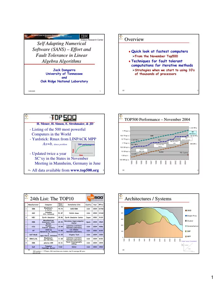
Architectures / Systems Architectures / Systems

100 200 300 400 500 1993 1994 1995 1996 1997 1998 1999 2000 2001 2002 2003 2004

S IMD S ingle Proc. Cluster Constellation S MP MPP

SLIDE 2

2

00 7

Top500 Performance by Manufacture (11/04)

IBM 49% HP 21%

• thers

14% SGI 7% NEC 4% Fujitsu 2% Cray 2% Hitachi 1% Sun 0% Intel 0%

00 8

Processor Types Processor Types

100 200 300 400 500

1993 1994 1995 1996 1997 1998 1999 2000 2001 2002 2003 2004 S IMD Vector S calar S parc MIPS intel HP Power Alpha 00 9

Interconnects / Systems Interconnects / Systems

100 200 300 400 500 1993 1994 1995 1996 1997 1998 1999 2000 2001 2002 2003 2004 Others Infiniband Quadrics Gigabit Ethernet Cray Int erconnect Myrinet S P S witch Crossbar N/ A

00 10

Fuel Efficiency: Fuel Efficiency: Gflops Gflops/Watt /Watt

0.1 0.2 0.3 0.4 0.5 0.6 0.7 0.8 0.9

BlueGene/L DD2 beta-System (0.7 GHz PowerPC 440) SGI Altix 1.5 GHz, Voltaire Infiniband Earth-Simulator eServer BladeCenter JS20+ (PowerPC970 2.2 GHz), Myrinet Intel Itanium2 Tiger4 1.4GHz - Quadrics ASCI Q - AlphaServer SC45, 1.25 GHz 1100 Dual 2.3 GHz Apple XServe/Mellanox Infiniband 4X/Cisco GigE BlueGene/L DD1 Prototype (0.5GHz PowerPC 440 w/Custom) eServer pSeries 655 (1.7 GHz Power4+) PowerEdge 1750, P4 Xeon 3.06 GHz, Myrinet eServer pSeries 690 (1.9 GHz Power4+) eServer pSeries 690 (1.9 GHz Power4+) LNX Cluster, Xeon 3.4 GHz, Myrinet RIKEN Super Combined Cluster BlueGene/L DD2 Prototype (0.7 GHz PowerPC 440) Integrity rx2600 Itanium2 1.5 GHz, Quadrics Dawning 4000A, Opteron 2.2 GHz, Myrinet Opteron 2 GHz, Myrinet MCR Linux Cluster Xeon 2.4 GHz - Quadrics ASCI White, SP Power3 375 MHz SP Power3 375 MHz 16 way TeraGrid, Itanium2 1.3/1.5 GHZ, Myrinet eServer Opteron 2.2 GHz. Myrinet xSeries Cluster Xeon 2.4 GHz - Quadrics eServer pSeries 655/690 (1.5/1.7 Ghz Power4+) xSeries Xeon 3.06 GHz, Quadrics eServer pSeries 690 (1.7 GHz Power4+) AIST Super Cluster P-32, Opteron 2.0 GHz, Myrinet Cray X1 eServer pSeries 690 (1.7 GHz Power4+)

Gflops/Watt Top 20 systems Based on processor power rating only

00 11

Fuel Efficiency: Fuel Efficiency: Gflops Gflops/Watt /Watt

0.1 0.2 0.3 0.4 0.5 0.6 0.7 0.8 0.9

BlueGene/L DD2 beta-System (0.7 GHz PowerPC 440) SGI Altix 1.5 GHz, Voltaire Infiniband Earth-Simulator eServer BladeCenter JS20+ (PowerPC970 2.2 GHz), Myrinet Intel Itanium2 Tiger4 1.4GHz - Quadrics ASCI Q - AlphaServer SC45, 1.25 GHz 1100 Dual 2.3 GHz Apple XServe/Mellanox Infiniband 4X/Cisco GigE BlueGene/L DD1 Prototype (0.5GHz PowerPC 440 w/Custom) eServer pSeries 655 (1.7 GHz Power4+) PowerEdge 1750, P4 Xeon 3.06 GHz, Myrinet eServer pSeries 690 (1.9 GHz Power4+) eServer pSeries 690 (1.9 GHz Power4+) LNX Cluster, Xeon 3.4 GHz, Myrinet RIKEN Super Combined Cluster BlueGene/L DD2 Prototype (0.7 GHz PowerPC 440) Integrity rx2600 Itanium2 1.5 GHz, Quadrics Dawning 4000A, Opteron 2.2 GHz, Myrinet Opteron 2 GHz, Myrinet MCR Linux Cluster Xeon 2.4 GHz - Quadrics ASCI White, SP Power3 375 MHz SP Power3 375 MHz 16 way TeraGrid, Itanium2 1.3/1.5 GHZ, Myrinet eServer Opteron 2.2 GHz. Myrinet xSeries Cluster Xeon 2.4 GHz - Quadrics eServer pSeries 655/690 (1.5/1.7 Ghz Power4+) xSeries Xeon 3.06 GHz, Quadrics eServer pSeries 690 (1.7 GHz Power4+) AIST Super Cluster P-32, Opteron 2.0 GHz, Myrinet Cray X1 eServer pSeries 690 (1.7 GHz Power4+)

Gflops/Watt Top 20 systems Based on processor power rating only

00 12

Fuel Efficiency: Fuel Efficiency: Gflops Gflops/Watt /Watt

0.1 0.2 0.3 0.4 0.5 0.6 0.7 0.8 0.9

BlueGene/L DD2 beta-System (0.7 GHz PowerPC 440) SGI Altix 1.5 GHz, Voltaire Infiniband Earth-Simulator eServer BladeCenter JS20+ (PowerPC970 2.2 GHz), Myrinet Intel Itanium2 Tiger4 1.4GHz - Quadrics ASCI Q - AlphaServer SC45, 1.25 GHz 1100 Dual 2.3 GHz Apple XServe/Mellanox Infiniband 4X/Cisco GigE BlueGene/L DD1 Prototype (0.5GHz PowerPC 440 w/Custom) eServer pSeries 655 (1.7 GHz Power4+) PowerEdge 1750, P4 Xeon 3.06 GHz, Myrinet eServer pSeries 690 (1.9 GHz Power4+) eServer pSeries 690 (1.9 GHz Power4+) LNX Cluster, Xeon 3.4 GHz, Myrinet RIKEN Super Combined Cluster BlueGene/L DD2 Prototype (0.7 GHz PowerPC 440) Integrity rx2600 Itanium2 1.5 GHz, Quadrics Dawning 4000A, Opteron 2.2 GHz, Myrinet Opteron 2 GHz, Myrinet MCR Linux Cluster Xeon 2.4 GHz - Quadrics ASCI White, SP Power3 375 MHz SP Power3 375 MHz 16 way TeraGrid, Itanium2 1.3/1.5 GHZ, Myrinet eServer Opteron 2.2 GHz. Myrinet xSeries Cluster Xeon 2.4 GHz - Quadrics eServer pSeries 655/690 (1.5/1.7 Ghz Power4+) xSeries Xeon 3.06 GHz, Quadrics eServer pSeries 690 (1.7 GHz Power4+) AIST Super Cluster P-32, Opteron 2.0 GHz, Myrinet Cray X1 eServer pSeries 690 (1.7 GHz Power4+)

Gflops/Watt Top 20 systems Based on processor power rating only

SLIDE 3

3

00 13 Chip (2 processors) Compute Card (2 chips, 2x1x1) 4 processors Node Card (32 chips, 4x4x2) 16 Compute Cards 64 processors System (64 racks, 64x32x32) 131,072 procs Rack (32 Node boards, 8x8x16) 2048 processors 2.8/5.6 GF/s 4 MB (cache) 5.6/11.2 GF/s 1 GB DDR 90/180 GF/s 16 GB DDR 2.9/5.7 TF/s 0.5 TB DDR 180/360 TF/s 32 TB DDR

IBM IBM BlueGene BlueGene/L /L

131,072 Processors 131,072 Processors

“Fastest Computer” BG/L 700 MHz 32K proc 16 racks Peak: 91.7 Tflop/s Linpack: 70.7 Tflop/s

77% of peak BlueGene/L Compute ASIC

Full system total of 131,072 processors

00 14

How Big Is Big? How Big Is Big?

♦ Every 10X brings new challenges 64 processors was once considered large

it hasn’t been “large” for quite a while

1024 processors is today’s “medium” size 8096 processors is today’s “large”

we’re struggling even here

♦ 100K processor systems are in construction we have fundamental challenges in dealing with machines of this size … and little in the way

• f programming support

00 15

Fault Tolerance: Motivation Fault Tolerance: Motivation

♦ Trends in HPC:

High end systems with thousand of processors

♦ Increased probability of a node failure

Most systems nowadays are robust

♦ MPI widely accepted in scientific computing

Process faults not tolerated in MPI model

Mismatch between hardware and (non fault- tolerant) programming paradigm of MPI.

00 16

Related work Related work

Manetho n faults [ EZ92] Egida [ RAV99] MPI / FT

Redundance of tasks

[ BNC01] FT- MPI

Modification of MPI routines User Fault Treatment

[ FD00] MPI CH-V

N faults Distributed logging

MPI - FT

N fault Centralized server

[ LNLE00]

Non Automatic Automatic

Pessim istic log Log based Checkpoint based Causal log Optim istic log ( sender based) Fram ew ork API Com m unication Layer Cocheck

I ndependent of MPI

[ Ste96] Starfish

Enrichment of MPI

[ AF99] Clip

Semi-transparent checkpoint

[ CLP97] Pruitt 9 8

2 faults sender based

[ PRU98] Sender based Mess. Log.

1 fault sender based

[ JZ87] Optim istic recovery I n distributed system s

n faults with coherent checkpoint

[ SY85]

A classification of fault tolerant message passing environments considering A) level in the software stack where fault tolerance is managed and B) fault tolerance techniques.

Causal logging + Coordinated checkpoint

LAM/MPI MPICH-V/CL LA-MPI

New community MPI effort OPEN-MPI

C^ 3

Compiler generated chkpt

[ Pingali, SC04]

00 17

FT FT-

• MPI

MPI http://icl.cs.utk.edu/ft

http://icl.cs.utk.edu/ft-

• mpi

mpi/ /

♦ Define the behavior of MPI in case an error

• ccurs.

♦ FT-MPI based on MPI 1.3 (plus some MPI 2

features) with a fault tolerant model similar to what was done in PVM.

Complete reimplementation, not based on other implementations.

♦ Gives the application the possibility to recover

from a process-failure.

♦ A regular, non fault-tolerant MPI program will

run using FT-MPI.

♦ What FT-MPI does not do:

Recover user data (e.g. automatic check-pointing) Provide transparent fault-tolerance

00 18

FT FT-

• MPI Failure Recovery Modes

MPI Failure Recovery Modes

♦ ABORT: Just do as other MPI

implementations.

♦ BLANK: Leave hole in

communicator.

♦ SHRINK: Re-order processes to

make a contiguous communicator.

Some ranks change

♦ REBUILD: Re-spawn lost

processes and add them to MPI_COMM_WORLD.

SLIDE 4

4

00 19

Fault Tolerance in the Fault Tolerance in the Computation Computation

♦ Some next generation systems

are being designed with > 100K processors (IBM Blue Gene L).

♦ MTTF 105 - 106 hours for

component.

sounds like a lot until you divide by 105! Failures for such a system can be just a few hours, perhaps minutes away. ♦ Problem with the MPI

standard, no recovery from faults.

FT-MPI allows user to provide recovery ♦ Application checkpoint /

restart is today’s typical fault tolerance method.

♦ Many cluster based on

commodity parts don’t have error correcting primary memory.

00 20

Fault Tolerance Fault Tolerance -

• Diskless Checkpointing

Diskless Checkpointing Built into Software Built into Software

♦

Checkpointing to disk is slow.

• May not have any disks on the system.

♦

Have extra checkpointing processors.

♦

Use “RAID like” checkpointing to processor.

♦

Maintain a system checkpoint in memory.

• All processors may be rolled back if necessary.
• Use k extra processors to encode checkpoints so that

if up to k processors fail, their checkpoints may be restored (Reed-Solomon encoding).

♦

Idea to build into library routines.

• We are looking at iterative solvers.
• Not transparent, has to be built into the algorithm.

00 21

How Raid for a Disk System Works How Raid for a Disk System Works

♦ Similar to RAID for disks.

♦ If X = A XOR B then this is true:

X XOR B = A A XOR X = B

00 22

How Diskless Checkpointing Works How Diskless Checkpointing Works

Comp Proc 1 Comp Proc p Check pt Proc

Data

Local Checkpoint

Data

Local Checkpoint Checkpoint Encoding

+

Memory Memory Memory

The encoding establishes an equality: C1 + C2 + … Cp = Cp+ 1. If one of the processor failed, the above equality becomes a linear equation with

• nly one unknown, therefore, lost data can be solved from the equation.

00 23

Diskless Checkpointing Diskless Checkpointing

♦ The N application processors

(4 in this case) each maintain their own checkpoints locally.

♦ K extra processors maintain

coding information so that if 1 or more processors fail, they can be replaced.

♦ Will describe for k=1 (parity). ♦ If a single processor fails,

then its state may be restored from the remaining live processors.

P0 P1 P3 P2 P4 P4 = P0 ƒ P1 ƒ P2 ƒ P3 Parity processor Application processors

00 24

Diskless Checkpointing Diskless Checkpointing

P0 P1 P3 P2 P4 P0 P3 P2 P4 P0 P3 P2 P4 P1 P4 takes on the identity of P1 and the computation continues. ♦ When failure occurs: control passes to user supplied handler “XOR” performed to recover missing data P4 takes on role of P1 Execution continue

SLIDE 5

5

00 25

A Fault A Fault-

• Tolerant Parallel Conjugate

Tolerant Parallel Conjugate Gradient Solver Gradient Solver

♦ Tightly coupled computation. ♦ Do a “backup” (checkpoint) every j iterations

for changing data.

Requires each process to keep copy of iteration changing data from checkpoint.

♦ First example can survive the failure of a single

process.

♦ Dedicate an additional process for holding data,

which can be used during the recovery

• peration.

♦ For surviving k process failures (k << p) you

need k additional processes (second example).

00 26

CG Data Storage CG Data Storage

Think of the data like this A b 3 vectors

Checkpoint A and b Initially, data is fixed throughout the iteration 3 vectors change every iteration

00 27

Parallel Version Parallel Version

Think of the data like this Think of the data like this

• n each processor

A b 3 vectors A b 3 vectors

. . . . . .

No need to checkpoint each iteration, say every j iterations. Need a copy of the 3 vectors from checkpt in each processor.

00 28

Diskless Version Diskless Version

P0 P1 P3 P2 P4 P0 P1 P2 P3 P4 Extra storage needed on each process from the data that is changing. Actually don’t do XOR, add the information.

00 29

FT PCG Algorithm Analysis FT PCG Algorithm Analysis

Global operation in PCG: three dot product, one preconditioning, and one matrix vector multiplication. Global operation in Checkpoint: encoding the local checkpoint. Global Operations

00 30

FT PCG Algorithm Analysis FT PCG Algorithm Analysis

Global operation in PCG: three dot product, one preconditioning, and one matrix vector multiplication. Global operation in Checkpoint: encoding the local checkpoint. Global operation in checkpoint can be localized by sub-group. Global Operations Checkpoint x, r, and p every k iterations

SLIDE 6

6

00 31

PCG: Test Problems (Matrices) PCG: Test Problems (Matrices)

bcsstk17 bcsstk17 bcsstk17

Bcsstk17: The size is: 10974 x 10974 Non-zeros: 428650 Sparsity: 39 non-zeros per row

• n average

Source: Linear equation from elevated pressure vessel

bcsstk17

Each process ow ns a block

00 32

PCG: Experiment Configurations PCG: Experiment Configurations

120 60 30 15

• No. of Comp. Procs

1,316,880 Problem #4 658,440 Problem #3 329,220 Problem #2 164,610 Problem #1 Size of the Problem

All experiment are performed on: 64 dual-processor 2.4 GHz AMD Opteron nodes Each node of the cluster has 2 GB of memory Each node runs the Linux operation system Nodes are connected with a Gigabit Ethernet.

00 33

PCG Performance with Different MPI Implementations 100 200 300 400 500 600 700 800 900 1000 Problem #1 Problem #2 Problem #3 Problem #4 Problems Time (Seconds) LAM-7.0.4 MPICH2-1.0 FT-MPI FT-MPI w/ ckpt FT-MPI w/ rcvr

PCG: Performance with Different MPI PCG: Performance with Different MPI Implementations Implementations

624.4 553.0 542.9 536.3

MPICH2-1.0

622.9 546.5 532.2 517.8

FT- MPI

624.4 547.8 533.3 518.9

FT-MPI ckpt /2000 iters FT-MPI exit 1 proc @10000 iters LAM- 7.0.4 T for 20000 iters

637.1 674.3 Problem #4 554.2 545.5 Problem #3 537.5 532.9 Problem #2 521.7 522.5 Problem #1

http://icl.cs.utk.edu/ft-mpi/

00 34

Protecting for More Than One Failure: Protecting for More Than One Failure: Reed Reed-

• Solomon (

Solomon (Checkpoint Encoding Matrices)

Checkpoint Encoding Matrices)

♦

In order to be able to recover from any k ( ≤ number of checkpoint processes ) failures, need a checkpoint encoding.

♦

With one checkpoint process we had:

P sets of data and a function A such that C=A*P where P=(P1,P2,…Pp)T;

C: Checkpoint data (C and Pi same size) With A = (1, 1, …, 1) C = a1P1 + a2P2 + …+ ap Pp; C = A*P To recover Pk; solve Pk = (C-a1P1-ak-1Pk-1– ak+1Pk+1– apPp)/ak

♦

With k checkpoints we need a function A such that

C=A*P where P=(P1,P2,…Pp)T;

C: Checkpoint data C = (C1,C2,…Ck)T (Ci and Pi same size). A: Checkpoint-Encoding matrix A is k x p (k << p).

♦

When h failures occur, recover the data by taking the h x h submatrix of A, call it A’, corresponding to the failed processes and solving A’P’ = C’; to recover the h “lost” P’s.

A’ is the h x h submatrix. C’ is made up of the surviving h checkpoints.

00 35

Reed Reed-

• Solomon Approach

Solomon Approach

A*P = C, where A is k x p made up of random numbers,

P is p x n, C is k x n Here using 4 processors and 3 Ckpt processors:

11 12 13 14 21 22 23 24 31 32 33 34

a a a a a a a a a a a a ⎛ ⎞ ⎜ ⎟ ⎜ ⎟ ⎜ ⎟ ⎝ ⎠

1 2 3 4

P P P P ⎛ ⎞ ⎜ ⎟ ⎜ ⎟ = ⎜ ⎟ ⎜ ⎟ ⎜ ⎟ ⎝ ⎠

1 2 3

C C C ⎛ ⎞ ⎜ ⎜ ⎜ ⎝ ⎠

00 36

A*P = C, where A is k x p made up of random numbers,

P is p x n, C is k x n Here using 4 processors and 3 Ckpt processors: Say 2 processors fail, P2 and P3.

11 12 13 14 21 22 23 24 31 32 33 34

a a a a a a a a a a a a ⎛ ⎞ ⎜ ⎟ ⎜ ⎟ ⎜ ⎟ ⎝ ⎠

1 2 3 4

P P P P ⎛ ⎞ ⎜ ⎟ ⎜ ⎟ = ⎜ ⎟ ⎜ ⎟ ⎜ ⎟ ⎝ ⎠

1 2 3

C C C ⎛ ⎞ ⎜ ⎜ ⎜ ⎝ ⎠

X X

Reed Reed-

• Solomon Approach

Solomon Approach

SLIDE 7

7

00 37

A*P = C, where A is k x p made up of random numbers,

P is p x n, C is k x n Here using 4 processors and 3 Ckpt processors: Say 2 processors fail, P2 and P3. Take a subset of A’s (colunm 2 and 3) and solve for P2 and P3.

11 12 13 14 21 22 23 24 31 32 33 34

a a a a a a a a a a a a ⎛ ⎞ ⎜ ⎟ ⎜ ⎟ ⎜ ⎟ ⎝ ⎠

1 2 3 4

P P P P ⎛ ⎞ ⎜ ⎟ ⎜ ⎟ = ⎜ ⎟ ⎜ ⎟ ⎜ ⎟ ⎝ ⎠

1 2 3

C C C ⎛ ⎞ ⎜ ⎜ ⎜ ⎝ ⎠

X X

12 13 2 1 22 23 3 2

a a P C a a P C ⎛ ⎞⎛ ⎞ ⎛ ⎞ = ⎜ ⎟⎜ ⎟ ⎜ ⎟ ⎝ ⎠ ⎝ ⎠⎝ ⎠

Reed Reed-

• Solomon Approach

Solomon Approach

Could use GF(2). Signal processing aps do this. In that case, A is Vandermonde

• r Cauchy matrix. (Need to have any

subset of A be non singular.) We use A as a random matrix.

00 38

PCG: Performance Overhead of Taking PCG: Performance Overhead of Taking Checkpoints Checkpoints

627.5 (4.2) 549.7 (3.2) 535.1 (3.0) 520.4 (2.8) 4 ckpt 624.4 (1.5) 547.8 (1.2) 533.3 (1.1) 518.9 (1.0) 1 ckpt 625.5 (2.3) 548.0 (2.0) 533.7 (1.8) 519.6 (1.7) 2 ckpt 626.7 (3.6) 548.8 (2.7) 534.5 (2.3) 519.8 (2.1) 3 ckpt 5 ckpt 0 ckpt T (ckpt T) 628.6 (4.5) 622.9 120 comp 550.1 (3.7) 546.5 60 comp 535.6 (3.5) 532.2 30 comp 521.0 (3.2) 517.8 15 comp Run PCG for 20000 iterations and take checkpoint every 2000 iterations (about 1 minute) PCG Performance Overhead for Taking Checkpoints 0.00% 0.20% 0.40% 0.60% 0.80% 1.00% 1.20% 15 30 60 120 Number of Computation Processors Checkpoint Overhead (%)

1 ckpt proc 2 ckpt proc 3 ckpt proc 4 ckpt proc 5 ckpt proc

00 39

PCG: Performance Overhead of PCG: Performance Overhead of Performing Recovery Performing Recovery

638.0 (12.0) 555.7 (8.2) 538.5 (5.7) 522.9 (3.7) 4 proc 637.1 (10.5) 554.2 (6.9) 537.5 (4.5) 521.7 (2.8) 1 proc 637.2 (11.1) 554.8 (7.4) 537.7 (4.9) 522.1 (3.2) 2 proc 637.7 (11.5) 555.2 (7.6) 538.1 (5.3) 522.8 (3.3) 3 proc 5 proc 0 proc T (ckpt T) 638.5 (12.5) 622.9 120 comp 556.1 (8.7) 546.5 60 comp 538.6 (6.1) 532.2 30 comp 523.1 (3.9) 517.8 15 comp Run PCG for 20000 iterations and take checkpoint every 2000 iterations (about 1 minute) Simulate a failure by exiting some processes at the 10000-th iteration PCG Performance Overhead for Performaning Recovery 0.00% 0.50% 1.00% 1.50% 2.00% 2.50% 15 30 60 120 Number of Computation Processors Recovery Overhead (%)

1 failed proc 2 failed proc 3 failed proc 4 failed proc 5 failed proc

00 40 PCG Perforamce Overhead for Checkpoint and Recovery 1 10 100 1000 60 120 240 480 Number of Computation Processors O ve rh e a d (S e co n d s)

T_ckpt T_rcvr_data T_rcvr_ftmpi

PCG: Preliminary Performance PCG: Preliminary Performance

Run PCG for 5000 iterations and take checkpoint every 1000 iterations (about 5 minutes) Simulate a failure of one node by exiting 4 processes at the 3000-th iteration. Matrix size scales with the processors used, i.e. 60 procs: n=658,440; 480 procs: n=5.2M 146.1 77.2 42.1 24.8 T_rcvr_ftmpi 1697.0 1557.5 1490.5 1441.7 T_tot 1531.1 1461.1 1429.3 1399.1 T_pcg_comp 9.7 9.2 9.2 8.0 T_ckpt 10.1 10.0 9.9 9.8 T_rcvr_dat a Time (Sec) 480 procs 240 procs 120 procs 60 procs

IBM RS/6000 SP w/176 Winterhawk II thin nodes (each with four 375 MHz Power3-II processors)

00 41

Predictive Adaptive Fault Predictive Adaptive Fault Tolerence Tolerence

♦ Large-scale fault tolerance

adaptation: resilience and recovery predictive techniques for probability of failure

resource classes and capabilities coupled to application usage modes

resilience implementation mechanisms

adaptive checkpoint frequency in memory checkpoints

♦ By monitoring, one can identify

performance problems failure probability

00 42

Next Steps Next Steps

Investigate ideas for 1K to 10K processors, then to BG/L.

♦ Software to determine the checkpointing interval and number of

checkpoint processors from the machine characteristics.

Perhaps use historical information. ♦ Local checkpoint and restart algorithm. Coordination of local checkpoints. Processors hold backups of neighbors. ♦ Have the checkpoint processes participate in the computation

and do data rearrangement when a failure occurs.

Use p processors for the computation and have k of them hold checkpoint. ♦ Generalize the ideas to provide a library of routines to do the

diskless check pointing.

♦ Look at “real applications” and investigate “Lossy” algorithms. ♦ FT-MPI available today and one of the contributions to Open

MPI.

SLIDE 8

8

00 43

Linpack (100x100) Analysis Linpack (100x100) Analysis

♦ Compaq 386/SX20 SX with FPA - .16 Mflop/s ♦ Pentium IV – 2.8 GHz – 1.3 Gflop/s ♦ 12 years we see a factor of ~ 8125 ♦ Moore’s Law says something about a factor of 2

every 18 months or a factor of 256 over 12 years

♦ Seem to be missing a factor of 32 …

Clock speed increase = 128x External Bus Width & Caching –

16 vs. 64 bits = 4x

Floating Point -

4/8 bits multi vs. 64 bits (1 clock) = 8x

Compiler Technology = 2x

♦ However the theoretical peak for that Pentium 4

is 5.6 Gflop/s and here we are only getting 1.3 Gflop/s

Still a factor of 4.25 off of peak

Complex set of interaction between Users’ applications Algorithm Programming language Compiler Machine instruction Hardware Many layers of translation from the application to the hardware Changing with each generation 00 44

Motivation Self Adapting Motivation Self Adapting Numerical Software (SANS) Effort Numerical Software (SANS) Effort

♦ Optimizing software to exploit the features of a

given system has historically been an exercise in hand customization. Time consuming and tedious Hard to predict performance from source code Must be redone for every architecture and compiler Software technology often lags architecture Best algorithm may depend on input, so some tuning may be needed at run-time. ♦ There is a need for quick/dynamic deployment

• f optimized routines.

00 45

Software Generation Software Generation Strategy Strategy -

• ATLAS BLAS

ATLAS BLAS

♦ Takes ~ 20 minutes to run,

generates Level 1,2, & 3 BLAS

♦ “New” model of high

performance programming where critical code is machine generated using parameter

• ptimization.

♦ Designed for modern

architectures

Need reasonable C compiler ♦ Today ATLAS in used within

various ASCI and SciDAC activities and by Matlab, Mathematica, Octave, Maple, Debian, Scyld Beowulf, SuSE,…

♦ Parameter study of the hw ♦ Generate multiple versions

• f code, w/difference

values of key performance parameters

♦ Run and measure the

performance for various versions

♦ Pick best and generate

library

♦ Level 1 cache multiply

• ptimizes for:

TLB access L1 cache reuse FP unit usage Memory fetch Register reuse Loop overhead minimization

♦

Similar to FFTW and Johnsson, UH

See: http://icl.cs.utk.edu/atlas/ joint with Clint Whaley & Antoine Petitet

0.0 500.0 1000.0 1500.0 2000.0 2500.0 3000.0 3500.0 A M D A t h l

• n
• 6

D E C e v 5 6

• 5

3 3 D E C e v 6

• 5

H P 9 / 7 3 5 / 1 3 5 I B M P P C 6 4

• 1

1 2 I B M P

• w

e r 2

• 1

6 I B M P

• w

e r 3

• 2

I n t e l P

• I

I I 9 3 3 M H z I n t e l P

• 4

2 . 5 3 G H z w / S S E 2 S G I R 1 i p 2 8

• 2

S G I R 1 2 i p 3

• 2

7 S u n U l t r a S p a r c 2

• 2

Architectures MFLOP/S

Vendor BLAS ATLAS BLAS F77 BLAS

00 46

Performance Tuning Methodology Performance Tuning Methodology

Input Parameters System specifics Hardware Probe Parameter study

• f code versions

Code Generation Performance database User options Installation

Software Installation

(done once per system)

♦

Parameter study of the hw

♦

Generate multiple versions of code, w/difference values of key performance parameters

♦

Run and measure the performance for various versions

♦

Pick best and generate library

♦

Optimize over 8 parameters

• Cache blocking
• Register blocking (2)
• FP unit latency
• Memory fetch
• Interleaving loads & computation
• Loop unrolling
• Loop overhead minimization

♦

Similar to FFTW Software Generation Software Generation Strategy Strategy -

• ATLAS BLAS

ATLAS BLAS http:// http://www.netlib.org www.netlib.org/atlas/ /atlas/

00 47

Self Adapting Numerical Software Self Adapting Numerical Software -

• SANS Effort

SANS Effort

♦ Provide software technology to aid in high performance on

commodity processors, clusters, and grids.

♦ Pre-run time (library building stage) and run time

• ptimization.

♦ Integrated performance modeling and analysis ♦ Automatic algorithm selection – polyalgorithmic functions ♦ Automated installation process ♦ Can be expanded to areas such as communication software

and selection of numerical algorithms

TUNING SYSTEM Different SW segment Size msgs “Best” SW segment Block msgs

00 48

Performance Tuning Methodology Performance Tuning Methodology

Input Parameters System specifics Hardware Probe Parameter study

• f code versions

Code Generation Performance database User options Installation

Software Installation

(done once per system)

Input Parameters Size, dim., … Select best algorithm Based on input data, State of hardware Cluster, etc Execution Data placement Calculate

Run-time

Performance Monitoring Database update

Software Execution

(done dynamically for each problem)

SLIDE 9

9

00 49

Real Crisis With HPC Is With The Real Crisis With HPC Is With The Software Software

♦ Programming is stuck

Arguably hasn’t changed since the 60’s

♦ It’s time for a change

Complexity is rising dramatically

highly parallel and distributed systems

From 10 to 100 to 1000 to 10000 to 100000 of processors!!

multidisciplinary applications

♦ A supercomputer application and software are usually

much more long-lived than a hardware

Hardware life typically five years at most. Fortran and C are the main programming models

♦ Software is a major cost component of modern

technologies.

The tradition in HPC system procurement is to assume that the software is free.

♦ We don’t have many great ideas about how to solve

this problem.

00 50

Some Current Unmet Needs Some Current Unmet Needs

♦ Performance / Portability ♦ Fault tolerance ♦ Better programming models

Global shared address space Visible locality

♦ Maybe coming soon (incremental, yet offering real

benefits):

Global Address Space (GAS) languages: UPC, Co-Array Fortran, Titanium)

“Minor” extensions to existing languages More convenient than MPI Have performance transparency via explicit remote memory references

♦ The critical cycle of prototyping, assessment, and

commercialization must be a long-term, sustaining investment, not a one time, crash program.

00 51

Collaborators / Support Collaborators / Support

♦ Top500 Team Erich Strohmaier, NERSC Hans Meuer, Mannheim Horst Simon, NERSC ♦ Fault Tolerant Work Julien Langou, UTK Jeffery Chen, UTK ♦ FT-MPI Graham Fagg, UTK Edgar Gabriel, HLRS Thara Angskun, UTK George Bosilca, UTK Jelena Pjesivac-Grbovic, UTK http://icl.cs.utk.edu/ft-mpi/