[PPT] - Optimal Design Scenario Problem: Definition and Evaluation of PowerPoint Presentation

SLIDE 1

Definition and Evaluation of Projected Hessians for Piggyback Optimization

Andreas Griewank, Nicolas Gauger, Jan Riehme Humboldt-Universit¨ at zu Berlin AD Workshop 2005, Nice, April 16

First •Prev •Next •Last •Full Screen •Close •Quit

AD Workshop 2005, Nice, April 16 1 Andreas Griewank, Nicolas Gauger, Jan Riehme, HU Berlin

Table of Content

General Scenario for Optimal Design
Single-step-one-shot = Piggy Back Optimization
Time-lagged derivative convergence for fixed u
Spectral analysis of single-step iteration
Numerical Result on Modified Bratu Example
Software and Implementation Issues on CFD Code
First •Prev •Next •Last •Full Screen •Close •Quit

AD Workshop 2005, Nice, April 16 2 Andreas Griewank, Nicolas Gauger, Jan Riehme, HU Berlin

Optimal Design Scenario

Problem:

Min f(y, u) s.t. c(y, u) = 0 where y ∈ Rm and u ∈ Rn are state and design variables

Available:

Code for f(y, u) and G(y, u) ≈ y −

∂

∂yc(y, u)

−1 c(y, u)

Assumption:

G, f ∈ C2,1(Rn+m) and ∂

∂yG(y, u) ≤ ρ < 1

Notation:

N(¯ y, y, u) ≡ f(y, u) + ¯ y G(y, u) ≡ Lagrangian + ¯ yy, where the Lagrangian is formed w.r.t. c(y, u) ≡ G(y, u) − y = 0.

First •Prev •Next •Last •Full Screen •Close •Quit

AD Workshop 2005, Nice, April 16 3 Andreas Griewank, Nicolas Gauger, Jan Riehme, HU Berlin

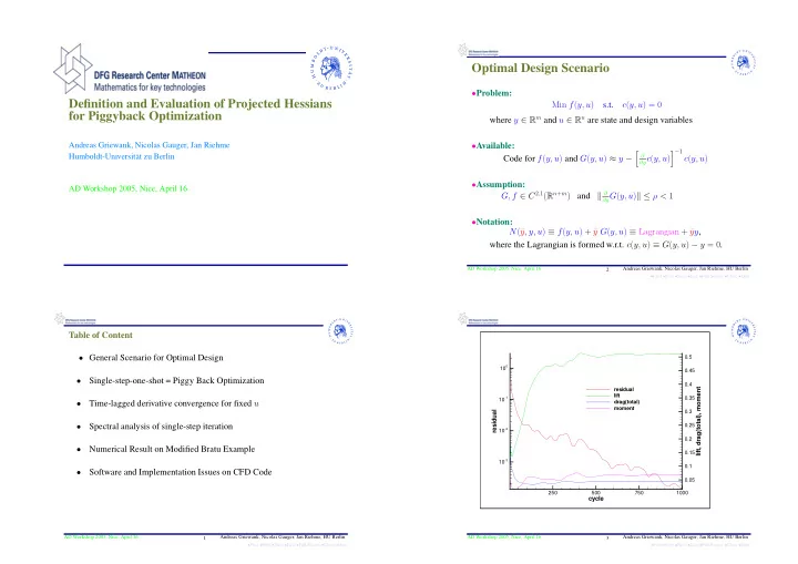
cycle residual lift, drag(total), moment

250 500 750 1000 10

3

10

2

10

1

10 0.05 0.1 0.15 0.2 0.25 0.3 0.35 0.4 0.45 0.5 residual lift drag(total) moment

SLIDE 2

First •Prev •Next •Last •Full Screen •Close •Quit

AD Workshop 2005, Nice, April 16 4 Andreas Griewank, Nicolas Gauger, Jan Riehme, HU Berlin

Single-step-one-shot = Piggy-Back Approach :

yk+1 = G(yk, uk) − → primal feasibility at y∗ ¯ yk+1 = Ny(yk, ¯ yk, uk) − → dual feasibility at ¯ y∗ uk+1 = uk − H−1

k Nu(yk, ¯

yk, uk) − → optimality at u∗ where Nu = ¯ y Gu + fu ≈ reduced gradient and Hk is a suitable preconditioner

First •Prev •Next •Last •Full Screen •Close •Quit

AD Workshop 2005, Nice, April 16 5 Andreas Griewank, Nicolas Gauger, Jan Riehme, HU Berlin

Questions/Tasks for Piggy-Back:

Avoid data objects larger than dim(y) · dim(u)
Analyse convergence of yk and ¯

yk for fixed u

Determine preconditioner Hk for fast local convergence
Evaluate/approximate Hk by differentiation or updating
Globalize by tradeoff between feasibility and optimality.
First •Prev •Next •Last •Full Screen •Close •Quit

AD Workshop 2005, Nice, April 16 6 Andreas Griewank, Nicolas Gauger, Jan Riehme, HU Berlin

Linear Convergence Result

Gy(y, u) − Gy(˜ y, u) ≤ νy − ˜ y ≥ fy(y, u) − fy(˜ y, u) = ⇒ lim k

∆yk

≤ ̺ ≥ lim k

∆¯

yk for ∆yk = yk − y(u) , ∆¯ yk = ¯ yk − ¯ y(u) Proof: Based on monotonic reduction of ∆yk + ω∆¯ yk for ω small enough.

First •Prev •Next •Last •Full Screen •Close •Quit

AD Workshop 2005, Nice, April 16 7 Andreas Griewank, Nicolas Gauger, Jan Riehme, HU Berlin

cycle residual

100 200 300 400 500 600 10

13

10

11

10

9

10

7

10

5

10

3

10

1

10

1

ONERA M6 Wing (mesh: 192x32x48 cells) MACH 0.840 ALPHA 3.1294 FLOWer, multigrid calculation (sym V-cycles on 3 mesh levels) green: primal solution red: adjoint solution

SLIDE 3

First •Prev •Next •Last •Full Screen •Close •Quit

AD Workshop 2005, Nice, April 16 8 Andreas Griewank, Nicolas Gauger, Jan Riehme, HU Berlin

Question: Do ∆yk and ∆¯ yk converge equally fast?? Answer: NO – Adjoints lag behind because: (G, f) ∈ C2,1, N(¯ y, y, u) ≡ ¯ yG(y, u) + f(y, u) = ⇒

∆yk+j

∆¯ yk+j

=
Gy

Nyy GT

y

j ∆yk ∆¯ yk

+ O (∆yk2 + ∆¯

yk2) = ⇒ provided Gy = TΓT −1, D = diag(T TBT)

Gy

Nyy GT

y

j ∼

Γj

jDT j−1 Γj

=

⇒ ∆¯ yk+j ≈ j̺j−1∆yk + ̺j∆¯ yk = ⇒ ∆yk/∆¯ yk∼ 1/k → 0.

First •Prev •Next •Last •Full Screen •Close •Quit

AD Workshop 2005, Nice, April 16 9 Andreas Griewank, Nicolas Gauger, Jan Riehme, HU Berlin

Consequence

Adjoints ¯ yk and reduced gradient ¯ uk ≡ Nu(¯ yk, yk, uk) − →

k

d f(y(u), u) du lag behind primal feasibility like 1

k. For fixed ˙

u also ˙ yk+1 = ˙ G(yk, ˙ yk, ˙ u) ≡ Gy(yk, uk) ˙ yk + Gu(xk, u) ˙ u and ˙ ¯ yk+1 ≡ ˙ ¯ G( ˙ yk, ¯ yk, ˙ yk, ˙ ¯ yk, u, ˙ u) = ˙ ¯ ykGy(yk, u)... converge, but lag behind according to ∆ ˙ yk∼ k∆yk and ∆ ˙ ¯ yk∼ k2∆yk

First •Prev •Next •Last •Full Screen •Close •Quit

AD Workshop 2005, Nice, April 16 10 Andreas Griewank, Nicolas Gauger, Jan Riehme, HU Berlin

18
16
14
12
10
8
6
4
2

500 1000 1500 2000 2500 3000 3500 4000 ln(step-norm) iterations k convergence history "sec-adj_.state" "adjoint_state" "direct._state" "original_state"

First •Prev •Next •Last •Full Screen •Close •Quit

AD Workshop 2005, Nice, April 16 11 Andreas Griewank, Nicolas Gauger, Jan Riehme, HU Berlin

50 100 150 200 250 300 350 500 1000 1500 2000 2500 3000 3500 4000 step-ratio iterations k error comparison "sec-adj_original" "adjoint_original" "direct_original"

SLIDE 4

First •Prev •Next •Last •Full Screen •Close •Quit

AD Workshop 2005, Nice, April 16 12 Andreas Griewank, Nicolas Gauger, Jan Riehme, HU Berlin

Test Problem:

Min f(y, u) ≡ 1

2

1

0 [(yn(ξ, 1) − 2.2)2 + σ(u(ξ)2 + u′(ξ)2)]dξ

s.t.

∆xy(x) + ey(x) = 0

for x ∈ [0, 1]2

Periodic boundary condition

y(0, ξ) = y(1, ξ)

for ξ ∈ [0, 1]

Dirichlet condition on lower edge

y(ξ, 0) = sin(2πξ)

for ξ ∈ [0, 1]

Boundary control on upper edge

y(ξ, 1) = u(ξ)

for ξ ∈ [0, 1]

Iteration Function

G ≡

(nonlinear) Jacobi-method on 5 points descretization.

First •Prev •Next •Last •Full Screen •Close •Quit

AD Workshop 2005, Nice, April 16 13 Andreas Griewank, Nicolas Gauger, Jan Riehme, HU Berlin

Spectral Analysis of Piggy-Back

∂(yk+1, ¯ yk+1, uk+1) ∂(yk, ¯ yk, uk) =   Gy Gu Nyy GT

y

Nyu −H−1Nuy −H−1GT

u I − H−1Nuu

  has at (y∗, ¯ y∗, u∗) as eigenvalues λ the roots of P(λ) ≡ det [H(λ) + (λ − 1)H] where H(λ) ≡ [Z(λ)T, I] ∇2

(y,u)N [Z(λ)T, I]T

Z(λ)T ≡ −GT

u(GT y −λI)−1

Rows of [Z(λ)T, I] span tangent space of {G(y, u) = λy}

First •Prev •Next •Last •Full Screen •Close •Quit

AD Workshop 2005, Nice, April 16 14 Andreas Griewank, Nicolas Gauger, Jan Riehme, HU Berlin

Contractivity in convex case

λ < 1 ⇐ ⇒ H ≻ 0 i.e. H pos. def. λ > −1 = ⇒ H ≻ H(−1)/2 Numerical experience on test problem above: Reduced Hessian H ≡ H(1) = ⇒ Immediate Blow-up Projected Hessian H ≡ H(−1) = ⇒ Full-step Convergence

First •Prev •Next •Last •Full Screen •Close •Quit

AD Workshop 2005, Nice, April 16 15 Andreas Griewank, Nicolas Gauger, Jan Riehme, HU Berlin                   34.90 −27.62 −1.11 −0.38 −0.15 −0.07 −0.06 −0.07 −0.15 −0.38 −1.11 −3.62 −27.62 58.90 −27.62 −1.11 −0.38 −0.15 −0.07 −0.06 −0.07 −0.15 −0.38 −1.11 −1.11 −27.62 58.90 −27.62 −1.11 −0.38 −0.15 −0.07 −0.06 −0.07 −0.15 −0.38 −0.38 −1.11 −27.62 58.90 −27.62 −1.11 −0.38 −0.15 −0.07 −0.06 −0.07 −0.15 −0.15 −0.38 −1.11 −27.62 58.90 −27.62 −1.11 −0.38 −0.15 −0.07 −0.06 −0.07 −0.07 −0.15 −0.38 −1.11 −27.62 58.90 −27.62 −1.11 −0.38 −0.15 −0.07 −0.06 −0.06 −0.07 −0.15 −0.38 −1.11 −27.62 58.90 −27.62 −1.11 −0.38 −0.15 −0.07 −0.07 −0.06 −0.07 −0.15 −0.38 −1.11 −27.62 58.90 −27.62 −1.11 −0.38 −0.15 −0.15 −0.07 −0.06 −0.07 −0.15 −0.38 −1.11 −27.62 58.90 −27.62 −1.11 −0.38 −0.38 −0.15 −0.07 −0.06 −0.07 −0.15 −0.38 −1.11 −27.62 58.90 −27.62 −1.11 −1.11 −0.38 −0.15 −0.07 −0.06 −0.07 −0.15 −0.38 −1.11 −27.62 58.90 −27.62 −3.62 −1.11 −0.38 −0.15 −0.07 −0.06 −0.07 −0.15 −0.38 −1.11 −27.62 34.90                                     69.81 −33.54 4.82 −2.81 1.88 −1.46 1.34 −1.46 1.88 −2.81 4.82 −9.54 −33.54 93.81 −33.54 4.82 −2.81 1.88 −1.46 1.34 −1.46 1.88 −2.81 4.82 4.82 −33.54 93.81 −33.54 4.82 −2.81 1.88 −1.46 1.34 −1.46 1.88 −2.81 −2.81 4.82 −33.54 93.81 −33.54 4.82 −2.81 1.88 −1.46 1.34 −1.46 1.88 1.88 −2.81 4.82 −33.54 93.81 −33.54 4.82 −2.81 1.88 −1.46 1.34 −1.46 −1.46 1.88 −2.81 4.82 −33.54 93.81 −33.54 4.82 −2.81 1.88 −1.46 1.34 1.34 −1.46 1.88 −2.81 4.82 −33.54 93.81 −33.54 4.82 −2.81 1.88 −1.46 −1.46 1.34 −1.46 1.88 −2.81 4.82 −33.54 93.81 −33.54 4.82 −2.81 1.88 1.88 −1.46 1.34 −1.46 1.88 −2.81 4.82 −33.54 93.81 −33.54 4.82 −2.81 −2.81 1.88 −1.46 1.34 −1.46 1.88 −2.81 4.82 −33.54 93.81 −33.54 4.82 4.82 −2.81 1.88 −1.46 1.34 −1.46 1.88 −2.81 4.82 −33.54 93.81 −33.54 −9.54 4.82 −2.81 1.88 −1.46 1.34 −1.46 1.88 −2.81 4.82 −33.54 69.81                  

SLIDE 5

First •Prev •Next •Last •Full Screen •Close •Quit

AD Workshop 2005, Nice, April 16 16 Andreas Griewank, Nicolas Gauger, Jan Riehme, HU Berlin

10
8
6
4
2

2 4 500 1000 1500 2000 2500 3000 ln(reduct-factor) iterations k convergence history "function" "lagrangian" "reduced_grad"

First •Prev •Next •Last •Full Screen •Close •Quit

AD Workshop 2005, Nice, April 16 17 Andreas Griewank, Nicolas Gauger, Jan Riehme, HU Berlin

12
10
8
6
4
2

2 500 1000 1500 2000 2500 3000 ln(step-norm) iterations k convergence history "sec-adj_.state" "adjoint_state" "direct._state" "original_state"

First •Prev •Next •Last •Full Screen •Close •Quit

AD Workshop 2005, Nice, April 16 18 Andreas Griewank, Nicolas Gauger, Jan Riehme, HU Berlin

Implicit calculation of H(λ) by additional iterations: Zk+1 = [Gy(yk, uk)Zk + Gu(yk, uk)]/ λ Z∗(1) ≡

dy∗ du ,

¯ Z∗(1) ≡

d¯ y∗ du

H∗(1) ≡

d¯ u∗ du

¯ Zk+1 = [Gy(yk, uk)T ¯ Zk + Nyy(yk, ¯ yk, uk)Zk + Nyu(yk, ¯ yk, uk)]

λ

Hk+1 = ¯ ZkGu(yk, uk) + Nuy(yk, ¯ yk, uk)Zk + Nuu(yk, ¯ yk, uk)

Convergence with contractive factor Gy/|λ| = ̺/|λ|.

First •Prev •Next •Last •Full Screen •Close •Quit

AD Workshop 2005, Nice, April 16 19 Andreas Griewank, Nicolas Gauger, Jan Riehme, HU Berlin

Tentative explanation:

Z(1) = (I − Gy)−1Gu is rich in monotonic modes, i.e. eigenvectors with eigenvalues close to 1. Z(−1) = (I + Gy)−1Gu is rich in alternating modes, i.e. eigenvectors with eigenvalues close to −1. It makes sense that the curvature of the Lagrangian with respect to the alternting modes is more critical than that with respect to the monotonic modes. If all eigenvalues of Gy were real the alternating modes could be eliminated by considering one double step G2(y, u) ≡ G(G(y, u), u)) as a single iteration. The resulting H(−1) would be much smaller. Working Hypothesis: Interesting iterations have complex eigenvalues.

SLIDE 6

First •Prev •Next •Last •Full Screen •Close •Quit

AD Workshop 2005, Nice, April 16 20 Andreas Griewank, Nicolas Gauger, Jan Riehme, HU Berlin

Implementation at the Software Level:

User supplied routine input: where: step(

↓

u,

↓

y, z

↓, f ↓

)

z= G(u,y)

utput:

f=f(u,y) Basic Iteration: init(u,z); y=0

while(y − z ≫ 0)

y=z step(u,y,z,f) use(z,f)

First •Prev •Next •Last •Full Screen •Close •Quit

AD Workshop 2005, Nice, April 16 21 Andreas Griewank, Nicolas Gauger, Jan Riehme, HU Berlin

Applying an AD tool in reverse mode: bstep(

(0)

bu

↓ , ↓

u,

(0)

by

↓

,

↓

y,

↓

bz, z

↓, ↓

bf, f

↓

) with: bu = Gu(y, u)Tbz + fu(y, u)Tbf by = Gy(y, u)Tbz + fy(y, u)Tbf Coupled basic and adjoint Iteration: init(u, z, by); y = 0; bz = 0 while(z − y + by − bz ≫ 0) y = z; bz = by; bu = 0; by = 0, bf = 1 bstep(bu, u, by, y, bz, z, bf, f) use(z, f, bu, by)

First •Prev •Next •Last •Full Screen •Close •Quit

AD Workshop 2005, Nice, April 16 22 Andreas Griewank, Nicolas Gauger, Jan Riehme, HU Berlin

One more differentiation in forward mode yields:. dbstep(

(0)

bu

↓ , ↓

u,

↓

du,

(0)

dbu

↓ , (0)

by

↓

,

↓

y,

↓

dy,

(0)

dby

↓

,

↓

bz, z

↓, dz ↓ , ↓

dbz,

↓

bf, f

↓

d f

↓

) Coupled basic with first and second adjoint : init(u, z, by, dz, dby); y = 0; bz = 0; dby = 0 while(z − y + by − bz + dz − dy + dby − dbz ≫ 0) y = z; bz = by, by = 0; bu = 0; dbu = 0; dby = 0 dy = dz/λ, dbz = dby/λ dbstep(bu, u, du, dbu, by, y, dy, dby, bz, z, dz, dbz, bf, fd f) use(z, f, bu, by, dbu, dby)

First •Prev •Next •Last •Full Screen •Close •Quit

AD Workshop 2005, Nice, April 16 23 Andreas Griewank, Nicolas Gauger, Jan Riehme, HU Berlin

Simplified Implementation:

User supplied routine input: where: step(

↓

u, y1 . . . y9, f

↓

)

y1 ...y9= G(u,y1...y9)

utput:

f=f(u,y) Basic Iteration: init(u)

while(???)

step(u,y1 ...y9,f) use(f)

SLIDE 7

First •Prev •Next •Last •Full Screen •Close •Quit

AD Workshop 2005, Nice, April 16 24 Andreas Griewank, Nicolas Gauger, Jan Riehme, HU Berlin

Simplified reverse mode:

bstep(

(0)

bu

↓ , ↓

u, by1 . . . by9, y1 . . . y9,

↓

bf, f

↓

)

Coupled basic and adjoint Iteration: init(u);

while(???)do bu = 0; bf = 1

bstep(bu, u, by1 . . . by9, y1 . . . y9, bf, f) use(f, bu) Same structure for second order adjoints =

⇒ preconditioners.

First •Prev •Next •Last •Full Screen •Close •Quit

AD Workshop 2005, Nice, April 16 25 Andreas Griewank, Nicolas Gauger, Jan Riehme, HU Berlin

0.3
0.2
0.1

0.1 0.2 0.3 0.4 0.6 0.8 1 1.2 1.4 1.6 mean line wing discritisation flow

First •Prev •Next •Last •Full Screen •Close •Quit

AD Workshop 2005, Nice, April 16 26 Andreas Griewank, Nicolas Gauger, Jan Riehme, HU Berlin 1e-07 1e-06 1e-05 0.0001 0.001 0.01 0.1 1 10 100 1000 100 200 300 400 500 600 700 800 900 residuum max{ubi - ubi-1} max{Hi - Hi-1}

First •Prev •Next •Last •Full Screen •Close •Quit

AD Workshop 2005, Nice, April 16 27 Andreas Griewank, Nicolas Gauger, Jan Riehme, HU Berlin

Iteration cos(angle(k,k+1)) L2-Residuals

25 50 75 100

1.1
1
0.9
0.8
0.7
0.6
0.5
0.4
0.3
0.2
0.1

10

4

10

3

10

2

10

1

10 rho: cos u: cos v: cos p: cos rho: L2 u: L2 v: L2 p: L2

SLIDE 8

First •Prev •Next •Last •Full Screen •Close •Quit

AD Workshop 2005, Nice, April 16 28 Andreas Griewank, Nicolas Gauger, Jan Riehme, HU Berlin

Summary and Conclusion

Sensitivities ’easily’ obtainable from fixed point solver
Storage requirement does not grow with iteration number
Derivatives converge also linearly but lag a little behind
Reduced Hessian no good preconditioner for single step piggy-backing
Optimal substep sequence and preconditioning depends on spectrum(Gy)
Preconditioning cost reducable to ≈ simulation step ????