Notes: UW RTG IPDE Summer School 2011 Finite Volume Methods and - PDF document

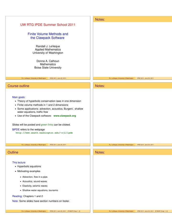
Notes: UW RTG IPDE Summer School 2011 Finite Volume Methods and the Clawpack Software Randall J. LeVeque Applied Mathematics University of Washington Donna A. Calhoun Mathematics Boise State University R.J. LeVeque, University of Washington IPDE 2011, June 20, 2011 R.J. LeVeque, University of Washington IPDE 2011, June 20, 2011 Course outline Notes: Main goals: • Theory of hyperbolic conservation laws in one dimension • Finite volume methods in 1 and 2 dimensions • Some applications: advection, acoustics, Burgers’, shallow water equations, traffic flow • Use of the Clawpack software: www.clawpack.org Slides will be posted and green links can be clicked. $IPDE refers to the webpage http://www.amath.washington.edu/~rjl/ipde R.J. LeVeque, University of Washington IPDE 2011, June 20, 2011 R.J. LeVeque, University of Washington IPDE 2011, June 20, 2011 Outline Notes: This lecture • Hyperbolic equations • Motivating examples • Advection, flow in a pipe. • Acoustics, sound waves • Elasticity, seismic waves • Shallow water equations, tsunamis Reading: Chapters 1 and 2 Note: Some slides have section numbers on footer. R.J. LeVeque, University of Washington IPDE 2011, June 20, 2011 [FVMHP Chap. 1, 2] R.J. LeVeque, University of Washington IPDE 2011, June 20, 2011 [FVMHP Chap. 1, 2]

Linear and nonlinear waves Notes: A wave is a disturbance or displacement that propagates. Examples: • Water waves (disturbance of depth) • Sound waves (disturbance of pressure) • Seismic waves (displacement of elastic material) Very small disturbances can be modeled by linear partial differential equations Solutions are often continuous, smooth functions Larger displacements require nonlinear equations Solutions may be discontinous: shock waves R.J. LeVeque, University of Washington IPDE 2011, June 20, 2011 R.J. LeVeque, University of Washington IPDE 2011, June 20, 2011 First order hyperbolic PDE in 1 space dimension Notes: q ( x, t ) ∈ lR m , A ∈ lR m × m Linear: q t + Aq x = 0 , f : lR m → lR m (flux) Conservation law: q t + f ( q ) x = 0 , Quasilinear form: q t + f ′ ( q ) q x = 0 Hyperbolic if A or f ′ ( q ) is diagonalizable with real eigenvalues. Models wave motion or advective transport. Eigenvalues are wave speeds. Note: Second order wave equation p tt = c 2 p xx can be written as a first-order system (acoustics). R.J. LeVeque, University of Washington IPDE 2011, June 20, 2011 [FVMHP Sec. 1.1] R.J. LeVeque, University of Washington IPDE 2011, June 20, 2011 [FVMHP Sec. 1.1] Derivation of Conservation Laws Notes: q ( x, t ) = density function for some conserved quantity, so � x 2 q ( x, t ) dx = total mass in interval x 1 changes only because of fluxes at left or right of interval. R.J. LeVeque, University of Washington IPDE 2011, June 20, 2011 [FVMHP Chap. 2] R.J. LeVeque, University of Washington IPDE 2011, June 20, 2011 [FVMHP Chap. 2]

Derivation of Conservation Laws Notes: q ( x, t ) = density function for some conserved quantity. Integral form: � x 2 d q ( x, t ) dx = F 1 ( t ) − F 2 ( t ) dt x 1 where F j = f ( q ( x j , t )) , f ( q ) = flux function . R.J. LeVeque, University of Washington IPDE 2011, June 20, 2011 [FVMHP Chap. 2] R.J. LeVeque, University of Washington IPDE 2011, June 20, 2011 [FVMHP Chap. 2] Derivation of Conservation Laws Notes: If q is smooth enough, we can rewrite � x 2 d q ( x, t ) dx = f ( q ( x 1 , t )) − f ( q ( x 2 , t )) dt x 1 as � x 2 � x 2 q t dx = − f ( q ) x dx x 1 x 1 or � x 2 ( q t + f ( q ) x ) dx = 0 x 1 True for all x 1 , x 2 = ⇒ differential form: q t + f ( q ) x = 0 . R.J. LeVeque, University of Washington IPDE 2011, June 20, 2011 [FVMHP Chap. 2] R.J. LeVeque, University of Washington IPDE 2011, June 20, 2011 [FVMHP Chap. 2] Advection equation Notes: Flow in a pipe at constant velocity u = constant flow velocity q ( x, t ) = tracer concentration, f ( q ) = uq = q t + uq x = 0 . ⇒ True solution: q ( x, t ) = q ( x − ut, 0) R.J. LeVeque, University of Washington IPDE 2011, June 20, 2011 [FVMHP Sec. 2.1] R.J. LeVeque, University of Washington IPDE 2011, June 20, 2011 [FVMHP Sec. 2.1]

Advection examples Notes: Here and on future slides, $IPDE refers to the webpage http://www.amath.washington.edu/~rjl/ipde $CLAW refers to the Clawpack top directory. Examples: • $IPDE/claw-apps/advection-1d-1 Created for this class. • $CLAW/apps/advection Example applications in Clawpack. • $CLAW/book Examples from the book. • www.clawpack.org/doc/apps.html Gallery of applications. R.J. LeVeque, University of Washington IPDE 2011, June 20, 2011 R.J. LeVeque, University of Washington IPDE 2011, June 20, 2011 Example: Linear acoustics in a 1d tube Notes: � p � p ( x, t ) = pressure perturbation q = u u ( x, t ) = velocity Equations: p t + κu x = 0 κ = bulk modulus ρu t + p x = 0 ρ = density or � p � � p � � � 0 κ + = 0 . u 1 /ρ 0 u t x � Eigenvalues: λ = ± c , where c = κ/ρ = sound speed Second order form: Can combine equations to obtain p tt = c 2 p xx R.J. LeVeque, University of Washington IPDE 2011, June 20, 2011 R.J. LeVeque, University of Washington IPDE 2011, June 20, 2011 Riemann Problem Notes: Special initial data: � q l if x < 0 q ( x, 0) = q r if x > 0 Example: Acoustics with bursting diaphram Pressure: Acoustic waves propagate with speeds ± c . R.J. LeVeque, University of Washington IPDE 2011, June 20, 2011 [FVMHP Sec. 3.9.1] R.J. LeVeque, University of Washington IPDE 2011, June 20, 2011 [FVMHP Sec. 3.9.1]

Riemann Problem for acoustics Notes: Waves propagating in x – t space: Left-going wave W 1 = q m − q l and right-going wave W 2 = q r − q m are eigenvectors of A . R.J. LeVeque, University of Washington IPDE 2011, June 20, 2011 [FVMHP Sec. 3.9.1] R.J. LeVeque, University of Washington IPDE 2011, June 20, 2011 [FVMHP Sec. 3.9.1] Seismic wave in layered medium Notes: Red = div(u) [P-waves], Blue = curl(u) [S-waves] R.J. LeVeque, University of Washington IPDE 2011, June 20, 2011 R.J. LeVeque, University of Washington IPDE 2011, June 20, 2011 Red = div(u) [P-waves], Blue = curl(u) [S-waves] Notes: Four levels with refinement factors 4, 4, 4 R.J. LeVeque, University of Washington IPDE 2011, June 20, 2011 R.J. LeVeque, University of Washington IPDE 2011, June 20, 2011

Shock formation Notes: For nonlinear problems wave speed generally depends on q . Waves can steepen up and form shocks = ⇒ even smooth data can lead to discontinuous solutions. Computational challenges! Need to capture sharp discontinuities. R.J. LeVeque, University of Washington IPDE 2011, June 20, 2011 R.J. LeVeque, University of Washington IPDE 2011, June 20, 2011 Shallow water equations Notes: h ( x, t ) = depth u ( x, t ) = velocity (depth averaged, varies only with x ) Conservation of mass and momentum hu gives system of two equations. mass flux = hu , momentum flux = ( hu ) u + p where p = hydrostatic pressure h t + ( hu ) x = 0 � hu 2 + 1 � 2 gh 2 ( hu ) t + = 0 x Jacobian matrix: � 0 1 � � f ′ ( q ) = , λ = u ± gh. gh − u 2 2 u R.J. LeVeque, University of Washington IPDE 2011, June 20, 2011 [FVMHP Sec. 13.1] R.J. LeVeque, University of Washington IPDE 2011, June 20, 2011 [FVMHP Sec. 13.1] Shallow water equations with bathymetry B ( x, y ) Notes: h t + ( hu ) x + ( hv ) y = 0 � hu 2 + 1 � 2 gh 2 ( hu ) t + + ( huv ) y = − ghB x ( x, y ) x � hv 2 + 1 � 2 gh 2 ( hv ) t + ( huv ) x + = − ghB y ( x, y ) y The equations have the form q t + f ( q ) x + g ( q ) y = ψ where � h � � hu � hu 2 + 1 2 gh 2 q ( x, y, t ) = hu , f ( q ) = , etc. hv huv R.J. LeVeque, University of Washington IPDE 2011, June 20, 2011 R.J. LeVeque, University of Washington IPDE 2011, June 20, 2011

DART buoy data Notes: Deep-ocean Assessment and Reporting of Tsunamis NOAA’s Network of pressure gauges on the ocean floor R.J. LeVeque, University of Washington IPDE 2011, June 20, 2011 R.J. LeVeque, University of Washington IPDE 2011, June 20, 2011 Notes: www.ndbc.noaa.gov/station_page.php?station=32412 R.J. LeVeque, University of Washington IPDE 2011, June 20, 2011 R.J. LeVeque, University of Washington IPDE 2011, June 20, 2011 DART buoy data Notes: R.J. LeVeque, University of Washington IPDE 2011, June 20, 2011 R.J. LeVeque, University of Washington IPDE 2011, June 20, 2011

NOAA unit sources for subduction zone Notes: From: Tang, L., V.V. Titov, and C.D. Chamberlin (2010): A Tsunami Forecast Model for Hilo, Hawaii. NOAA OAR Special Report, PMEL Tsunami Forecast Series: Vol. 1, 94 http://nctr.pmel.noaa.gov/pubs.html R.J. LeVeque, University of Washington IPDE 2011, June 20, 2011 R.J. LeVeque, University of Washington IPDE 2011, June 20, 2011 Response at DART buoy from unit earthquakes Notes: Propagation in deep water is essentially linear... Fit linear combination of these responses to DART data. R.J. LeVeque, University of Washington IPDE 2011, June 20, 2011 R.J. LeVeque, University of Washington IPDE 2011, June 20, 2011 Best fit from unit earthquakes Notes: Best fit with constraint that all coefficients (dislocations) positive. R.J. LeVeque, University of Washington IPDE 2011, June 20, 2011 R.J. LeVeque, University of Washington IPDE 2011, June 20, 2011