
SLIDE 1
Outline
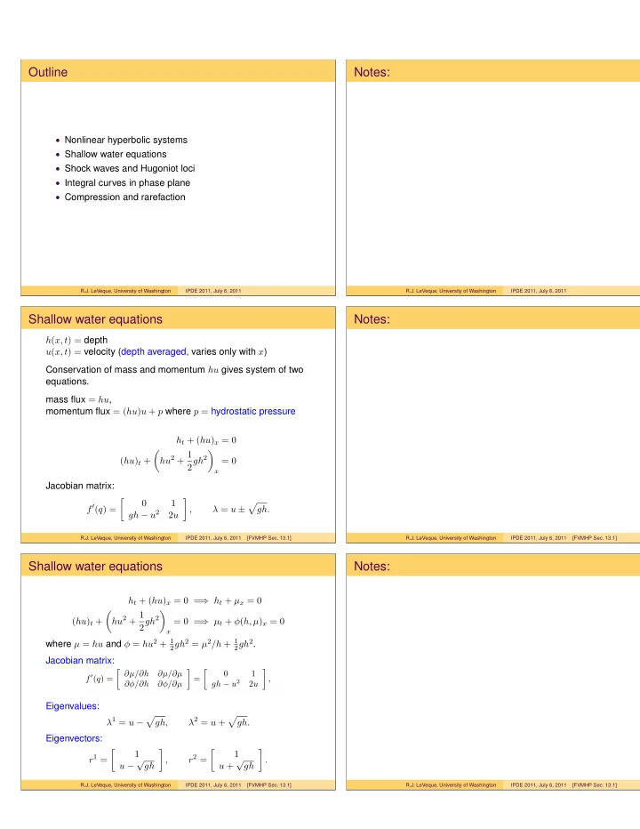
- Nonlinear hyperbolic systems
- Shallow water equations
- Shock waves and Hugoniot loci
- Integral curves in phase plane
- Compression and rarefaction
R.J. LeVeque, University of Washington IPDE 2011, July 6, 2011
Notes:
R.J. LeVeque, University of Washington IPDE 2011, July 6, 2011
Shallow water equations
h(x, t) = depth u(x, t) = velocity (depth averaged, varies only with x) Conservation of mass and momentum hu gives system of two equations. mass flux = hu, momentum flux = (hu)u + p where p = hydrostatic pressure ht + (hu)x = 0 (hu)t +
- hu2 + 1
2gh2
- x
= 0 Jacobian matrix: f′(q) =
- 1
gh − u2 2u
- ,
λ = u ±
- gh.
R.J. LeVeque, University of Washington IPDE 2011, July 6, 2011 [FVMHP Sec. 13.1]
Notes:
R.J. LeVeque, University of Washington IPDE 2011, July 6, 2011 [FVMHP Sec. 13.1]
Shallow water equations
ht + (hu)x = 0 = ⇒ ht + µx = 0 (hu)t +
- hu2 + 1
2gh2
- x
= 0 = ⇒ µt + φ(h, µ)x = 0 where µ = hu and φ = hu2 + 1
2gh2 = µ2/h + 1 2gh2.
Jacobian matrix:
f ′(q) = ∂µ/∂h ∂µ/∂µ ∂φ/∂h ∂φ/∂µ
- =
- 1
gh − u2 2u
- ,
Eigenvalues: λ1 = u −
- gh,
λ2 = u +
- gh.
Eigenvectors: r1 =
- 1
u − √gh
- ,
r2 =
- 1
u + √gh
- .
R.J. LeVeque, University of Washington IPDE 2011, July 6, 2011 [FVMHP Sec. 13.1]
Notes:
R.J. LeVeque, University of Washington IPDE 2011, July 6, 2011 [FVMHP Sec. 13.1]